Chapter 5
Inference Methodology

Highly multivariate data is often challenging to model due to the “curse of dimensionality” Bellman (1957). Much of the work in this thesis is concerned with reducing the computational burden associated with modelling the response of vegetation to climate using the modern training data (see Section 1.1.1).

This is achieved through separate analysis of the marginal responses of individual plant taxa to climate. The approach necessarily ignores between taxa dependencies but allows for reduction of overall computation. The separate, marginal analyses can then be brought together post-hoc. This is referred to as the inference-via-marginals posterior and is an approximation to the joint posterior of the full model. Situations where the approximation is poor and where it is excellent, or even exact, are identified.

Details related to working on a discrete grid across the location space are also investigated. This chapter serves as a review and assessment of the preceding chapters methodology. The methods are brought together in preparation for the application to the pollen dataset in Chapter 6.

In particular, the concern here is with inference on multiple latent spatial Gaussian processes defined on a lattice. The INLA methodology introduced in Section 4.1 is unsuitable for this task as it can only deal with one such spatial process at a time (see Section 5.1.4). If the model does not disjoint-decompose (Section 3.2) exactly then approximations to the model that do decompose must be sought. The accuracy of these approximations must then be tested, as per Section 5.3.

The goal is inference on latent random variables X, given counts data Y defined at discrete locations C. X is composed of N_T processes which are Gaussian (or approximately so) given the data. Thus at each value of C, there are N_T counts or proportions arising from N_T potentially dependent X values. As the posterior is GMRF due to the methods introduced in Section 4.1, it is expressed via the posterior mean vector μ and precision matrix Q. i.e. the posterior distribution of X is given approximately by:

(5.1)

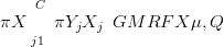
The goal is therefore inference on the μ and Q terms. By disjoint-decomposition into marginals defined as the product of independent multivariate X_i,i 1,…,N_T across locations C becomes:

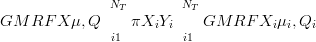(5.2)

The INLA method then delivers the terms μ_i and Q_i that define the independent spatial X_i given the data. The error incurred due to this decomposition is the subject of Section 5.3.

5.1 Reasons for Disjoint-Decomposition

5.1.1 Parallelisation

If the overall problem disjoint-decomposes (see Section 3.2) then the exploitation of parallel programming resources is trivial. Inference on each disjoint module may be performed entirely independently of the others and thus may be done at the same time on multiple processors. No specialist code or hardware is required and joint summary statistics are simple and quick calculations that are made on a single processor.

5.1.2 Memory Usage

When responses are modelled non-parametrically (see Section 1.1.1) as for the palaeoclimate dataset, the number of parameters is of the order of 10³ for a two dimensional climate space. Ultimately, the goal is to work with at least three climate variables (leading to the order of millions of parameters) and also to integrate out the unknown hyperparameters. The memory required simply to store such a burdensome model may quickly overwhelm even modern, high specification personal computers.

Memory usage is therefore one of the most difficult issues associated with performing inference on this dataset. It is crucial to reduce both the computational overhead and the size the model takes up in memory. Breaking the model down into a series of approximately disjoint / conditionally independent marginals negates the need to store and manipulate all of the parameters at once on a single machine.

5.1.3 Inverse Problem

Another large saving in terms of computation is in the inversion of the forward model; a high dimensional integral (to find the joint marginal likelihood) is replaced with a product of uni-dimensional integrals. These may be evaluated without resorting to Monte-Carlo based sampling methods that are required for the estimation of multidimensional integrals.

5.1.4 Compatibility with the INLA Method

If the joint model does not decompose, then inference must be performed for the entire model at once. Interaction terms between marginals are non-zero and must be modelled explicitly. For problems consisting of multiple smooth surfaces giving rise to vectors of counts, such as the motivating palaeoclimate problem, this results in difficulties for the INLA inference method.

Interaction may occur at one of two levels in the model hierarchy; either in the prior or the likelihood. The former models smooth surfaces that are not independent across locations; the latter models independent smooth surfaces that jointly give rise to non-independent counts. This is a continuation of the discussion in Section 3.2.2.

Prior and Hyperparameters

If the interactions between marginals are modelled at the latent variable stage, then the joint prior must contain these terms. Specifically, the joint prior precision matrix must contain non-zero terms for the interactions. If they are not known a-priori then unknown hyperparameters must be introduced to model these inter-process precisions.

The INLA method deals with hyperparameters via numerical integration. The entire vector of hyperparameters is set on a discrete grid, as per Section 4.1.3. This approach requires that the number of hyperparameters is low; any more than five or so and the method runs into computational difficulty. The motivating palaeoclimate problem has 28 plant taxa; even crude modelling of the interactions with a single hyperparameter governing each taxon-taxon interaction results in 378 additional hyperparameters; this is far more than the INLA method can cope with (Rue et al. (2008)).

Likelihood and Taylor Expansions

Modelling the interactions at the data level eliminates the need for additional interaction hyperparameters. Interaction terms are placed in the likelihood precision matrix and are thus parameters rather than hyperparameters; however the data are not conditionally independent. The Taylor series expansions in the GMRF approximation are no longer univariate, resulting in a massive increase in the computation required to fit the approximation (see Section 4.1.2). This is a fundamental challenge to the existing INLA methodology.

5.2 Multivariate Normal Model

Much of this chapter focusses on the marginal analysis of data in a Gaussian setting. The reasons for exploration of such a problem in a purely Gaussian framework are as follows:

1. For simple exploration and illustration of key points; the availability of the posterior in closed form is the primary motivation.
2. For synthesis with the Gaussian approximation technique described in Section 4.1. This technique applies a Gaussian prior and approximates the posterior with a Gaussian.

Given a multivariate normal prior πX and multivariate normal likelihood πY SX, the posterior πXSY is multivariate normal with mean and precision matrix given by

where the prior precision matrix is Q_X and the likelihood precision matrix is Q_Y .

5.2.1 Conditions for Perfect Disjoint-Decomposition

If the joint posterior expresses zero precision between processes then a fully joint inference may be done exactly via the marginals. There are in fact two situations in which this occurs:

1. The underlying processes are truly independent of each other
2. The joint model creates a posterior with conditional independence across the latent variables, regardless of any dependency structure suggested by the data ¹

The second situation for a perfect inference-via-marginals is clearly illustrated with two common examples. These are discussed in Section 5.2.2 and Section 5.2.

The terminology used in this thesis will be that the joint model disjoint-decomposes exactly (see Section 3.2).

It can immediately be seen from Equation (5.3) that the condition for exact disjoint-decomposition of the posterior is that both the prior and the likelihood disjoint-decompose. The form of the precision matrix shows whether a density will decompose; if it is block-diagonal, then the blocks each represent a disjoint part of the full model. See Table 5.1 for illustration.

The assumption that the precision of process i₁ at location j₁ given process i₂ at location j₂ ( j₁ is zero is logical; there will not be interaction between a plant taxon at one climate location and a different taxon at another, disparate location in climate space. This results in a banded overall precision matrix and is similar to the Separable Models described in Finkenstdt et al. (2006). However, their approach cannot be exploited here. Separable models involve modelling two separate precision matrices; typically a spatial matrix and a temporal matrix. The spatio-temporal precision matrix is then taken as the Kronecker product of these two matrices. Taking a Kronecker product of an intra-process precision matrix and an inter-process precision matrix would impose two modelling aspects that are unsuitable for this work. Specifically, (i) implementation of a separable model would require using a common spatial precision matrix for all processes and (ii) would lead to non-zero _i1,j1^i₂,j₂ terms in the precision matrices for i₁ ( i₂ and j₁ ( j₂.

5.2.2 Compositional Independence

Although it would seem that compositional data analysis must necessarily model interaction between the components of the composition (in the pollen dataset, the components are the various plant taxa), Aitchison demonstrates that any statistical analysis making use of the Dirichlet distribution is in fact imposing a strong implied independence structure (Aitchison (1986) 3.4). Similarly, any logistic-normal (Section 3.5.4) distribution with diagonal precision matrix will impose the same strong implied independence structure.

For example, in a Bayesian setting, joint inference done on the latent vector of probability parameters P governing a compositional counts vector Y might proceed as follows:
Likelihood is Multinomial:

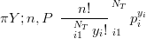(5.4)

where n P_iY _i
Prior is Dirichlet

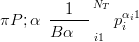(5.5)

where α is a vector of hyperparameters
The posterior is then Dirichlet due to conjugacy

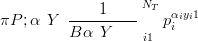(5.6)

The vector P is subject to the constraint that P_iP_i 1 and the vector of counts Y is subject to the constraint that P_iY _i n.

However, the Multinomial and the Dirichlet actually enforce conditional independence given the constraints.

The Multinomial can be expressed as a product of Poisson distributions, with parameters equal to nP, conditioned on the sum being equal to the total count n. This sum (P_iy_i n) itself follows a Poisson distribution with rate parameter n.

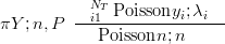(5.7)

with λ_i n p_i and Poissony_i;λ_i

Similarly, a Dirichlet with parameter vector η may be expressed as a product of Gamma distributions, with shape parameters η and rate parameters all equal to P_iη_i, conditioned on the sum = 1 following a Gamma distribution with shape and rate both equal to P_iη_i.

(5.8)

Therefore, to perform joint inference given a vector of counts and using a Dirichlet prior and a Multinomial likelihood, no accuracy is lost in performing marginal inferences on each part of the composition and then conditioning on the sum. This result is regardless of the value of the parameters of the distributions.

If sampling from the Dirichlet posterior is required, this can be achieved by sampling from the Gamma marginals and then rescaling such that the sum is one. In fact, this is the usual algorithm for sampling from a Dirichlet distribution. The post-hoc conditioning or rescaling is the only step that requires joint knowledge of the marginals.

5.3 Sensitivity to Inference via Marginals

If the joint model disjoint-decomposes then the inference-via-marginals approximation is exact. If not, the approximation amounts to setting non-zero terms in the overall precision matrix to be zero. This is equivalent to breaking some links in the graph of the model, specifically the inter-process links.

The accuracy of the inference-via-marginals approximation depends on several factors. The magnitude of the non-zero terms that are set to zero to facilitate decomposition are the most obvious of these. The further these are from zero, the greater the interaction and hence the worse the inference-via-marginals approximation will be. However, given non-zero interactions, several other factors will impact the level of accuracy.

Ultimately, the interest is in the differences between a full joint model and the inference-via-marginals model in terms of the inverse problem. Of course, if the forward model disjoint-decomposes exactly, then the inverse predictive distributions will be identical for the two models.

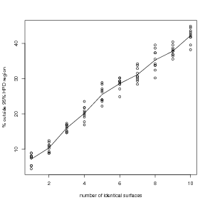
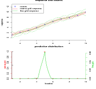
The worst case scenario is presented in Figure 5.1. A single surface is replicated T times; random counts are generated at various points in the location space. Inverse cross-validation predictive distributions are formed and the joint predictive distribution is found by taking the product and normalising (see Section 3.2). However, this model treats the surfaces as independent; they are in fact fully correlated. This results in a linear increase with Δ, the percentage of points lying outside their 95% cross-validation highest inverse predictive density with T.

Thus the inference-via-marginals model is a poor approximation; correlation of 1 between the surfaces (as they are all identical) represents the upper bound of inaccuracy of the inference-via-marginals approximation. Even if the data are simulated for each replication of the surface independently, the model does not disjoint-decompose.

To see this, take s₁c s₂c both the same smooth function of c. Random samples x₁ Ns₁,ϵ and x₂ Ns₂,ϵ will have high corrx₁,x₂ but low corrx₁,x₂Sc. So inference on the forward model may be completed marginally. Thus the result in Figure 5.1 is, at first glance, counter-intuitive. Independent counts should yield a tighter predictive density on the correct location. Δ should converge to zero as the predictive cross-validation densities converge to Dirac distributions on the correct locations.

The reason why this is not so is a peculiarity of the inverse problem; the shape of the response surface in this case is such that for any given location, there is typically one or more other locations with the same (or a very similar) value for the response. When a point is left out, the posterior variance at that point is greater than the locations for which there is data (for illustration, see Figure 2.3(b)). Thus the marginal likelihood is higher for these other locations; in turn the inverse predictive density will give greater weight to those locations with data and a similar response to the correct location. For a single response surface, this does not cause a problem. It is when analysing multiple surfaces that the issue arises.

Although the correct, left-out location has non-zero predictive density for a single surface (and is within the bounds of the 95% highest posterior predictive density 95% of the time), it will tend to zero as T increases. Multiplication of the density with itself T times will cause the location with the single highest density to gain all the mass as the number of replications of the surface increases. Thus, the correct location loses predictive probability mass and Δ increases.

In the simplest example, suppose inference on a single surface leads to the (correct) location predictive density of 75% probability mass a location A and 25% at location B, with location B the correct location. This is ok in terms of the Δ statistic; B is within the 95% HPD region. Now suppose that we are presented with new data from the same response, but treat it as independent. We might find, again without error, that this data suggests PA 70% and PB 30%. Again, this is ok. Assumption that the data are independent however, leads to a multiplication and re-normalisation of these values so that PA 87.5% and PB 12.5%. A third dataset yields PA 80% and PB 20%. The resultant multiplicative joint predictive distribution then has PA 96.55% and PB 3.45%. Now B is outside the 95% HPD region.

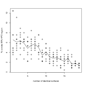
This issue will not arise when there is no other region of the location space with a very similar counts data vector. Using the exact same model and code used to produce Figure 5.1, but generating a new random response surface for each replication results in a Δ statistic of exactly zero for 20 surfaces. This is because each surface carries independent information on the location given counts data. Figure 5.2 shows a plot of ΔT for random independent surfaces.

Note that this convergence to a probability of one at the correct location will also occur for the case of replicated identical surfaces when the cross-validation is performed using the saturated posterior.

5.3.1 Discrete HPD Regions

The reason why Δ does not converge to 5% and instead converges to 0% as the number of conditionally independent counts increases is due to the discrete grid. As per Section 3.1.3, the HPD region contains 95% or more of the total probability mass. Therefore, the expected value of Δ is B 5% for each independent surface.

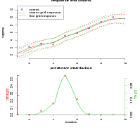
As more of these conditionally independent components are brought together, each with Δ B 5%, the predictive distributions become increasingly peaked. They are centred on the correct location (under the correct model) and so the probability mass becomes focused at the correct location. Eventually, the 95% HPD region becomes smaller than the grid spacing so that all the mass is concentrated on a single gridpoint. Using the algorithm in Section 3.1.3 for constructing discrete 95% HPD regions then results in selection of the single gridpoint that contains all this mass. As this is the correct location, none of the points lie outside their corresponding 95% (or more) HPD region and Δ tends to zero. A graphic illustration of this phenomenon is presented in Figure 5.3.

(a) 2 counts per location (b) 20 counts per location Fig. 5.3: UPPER PANELS: A linear response gives rise to Gaussian counts (blue circles). If there are n independent counts at each location, this is analagous to multiple conditionally independent counts. These counts data are used to inform the mean posterior response on a coarse grid (red line) and fine grid (green line) and posterior variances (the broken lines depict the mean response 2σ with σ the posterior standard deviation). LOWER PANELS: As the number of independent observations increases, the inverse predictive distribution becomes sharper; a mean count of 5 given 2 counts (Figure (a)) gives rise to a broader predictive distribution than a mean count of 5 given 20 counts (Figure (b)). The probability mass on the coarse grid is depicted without joining the points (red circles). The fine grid approximates continuous space and so a line is used. Although the coarse and fine grids deliver similar results at the coarse gridpoints (subject to the difference in scale due to the differing number of evaluation points), Figure (b) shows how the 95% HPD region will differ. The coarse grid now concentrates all mass at a single point. Hence the discrete 95% or greater HPD region will actually converge to a 100% HPD region and the Δ statistic converges to 0%.

5.3.2 Nested Constrained Models

Nested constrained models represent an interesting opportunity to apply disjoint-decomposition to a joint model that does not decompose exactly as the product of its marginals (see Section 3.5.6).

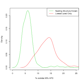
Given knowledge of the nesting structure, the joint model may be exactly expressed as the product of the marginals across all levels of the nesting hierarchy, where the dependencies within levels are accounted for in the likelihood using knowledge of the counts and responses of higher levels in the structure.

The advantage of such models is that they will disjoint-decompose iff nesting structure is known a-priori. If the nesting is not known, the marginals model at the lowest level only will be a poor fit to the data. Figure 5.4 shows results for inference-via-marginals models fitted to the same data-sets used in Figure 3.14, but with the added task of inference of the forward model. It is clear that attempting to model the joint model as the product of the marginals without exploitation of the nesting structure results in a poor model fit. In contrast, knowledge of the nesting structure allows for exact disjoint-decomposition of the model.

5.4 Conclusions

Inference on multivariate models comprised of multiple spatial processes may be performed in disjoint modules; provided there is no interaction between these modules in either the prior or the likelihood. Decomposition is into the marginals for each process.

The multivariate normal setting delivers insight into more general models, where the posteriors may be approximated with a GMRF. This approximation requires that the model decomposes. If it does not, then use of a disjoint-decomposable model is equivalent to a model with the interaction terms set to zero. This is an approximation, the accuracy of which is determined by the degree of correlation between the marginals. When such correlation is non-zero, the loss in accuracy increases linearly with the number of non-independent processes. Accuracy here is measured by the percentage of points lying outside their 95% discrete HPD region under leave-one-out cross-validation inverse predictive distributions.

Compositional models, in which both the data and the likelihood parameters are constrained under summation, represent a class of model that do not decompose. However, many compositional models do decompose for inference on the model parameters, subject to a post-hoc conditioning or rescaling. Compositional models which do not disjoint-decompose may in do so given knowledge of a nesting structure. Such structures must be known a-priori to facilitate decomposition of the model.