Chapter 1
Introduction
Highly multivariate statistical problems may lead to slow inference procedures. One
example of such a problem involves palaeoclimate reconstruction from fossil pollen data,
which is an example of an inverse problem. Existing explorations of this challenging
area of study often involve a trade off between model complexity and speed
of inference. Fast approximate Bayesian inference methods offer a solution. In
addition, an extension of the methodology allows for model validation to be
performed quickly for the inverse problem. Conversely, the large scale of the
palaeoclimate project offers a real challenge to the emerging approximate inference
engine.
The Royal Statistical Society read paper “Bayesian Palaeoclimate Reconstruction”,
Haslett et al. (2006) presented work on high resolution pollen based reconstruction of the
palaeoclimate at a single location since the last ice-age. This paper outlined the basic
concepts involved in performing fully Bayesian inference on unknown climates
given modern and fossil pollen data and modern climatic data. The work was
a detailed “proof of concept”; extensions and improvements to the statistical
methodology were considered, both in the paper and in the subsequent printed
discussion.
The main crux of the methodology in that work was acknowledged to be
computational; indeed the computational burden imposed compromises on the modelling.
The work presented herein represents extensions in the statistical methodology and
advances in the computations involved as developed by the author. These contributions
are outlined in Section 1.4.
1.1 Palaeoclimate Reconstruction Project
The Bayesian palaeoclimate reconstruction project is an ongoing initiative to build upon
existing classical approaches to the reconstruction of prehistoric climates, using fossil
pollen data. Specifically, the project seeks to handle all uncertainties quantitatively and
coherently in a fully Bayesian framework and to combine different types of information to
reduce these uncertainties.
1.1.1 The RS10 Pollen Dataset
The primary dataset for the palaeoclimatology reconstruction project is the RS10
dataset of Allen et al. (2000). A collection of modern pollen surface sample counts
Y m ��y1m,…,yMm�;M � 7742 are taken from the uppermost 5 to 10mm of lake bed
sediment at numerous locations in the northern hemisphere. Along with covariates in the
form of local contemporary climate measurements Lm, they comprise the modern dataset.
This is also referred to as the training data. Sample fossil pollen counts Y f are extracted
from cores taken from lake or mire sediment. Measures of the prehistoric climate variables
Lf at the time of deposition of these fossil pollen spores are unknown; the central
premise of palynological palaeoclimate reconstruction is that these climates
may be inferred from the pollen data, albeit with some uncertainty. Both the
modern and fossil pollen data comprise counts of numerous plant types (taxa; see
below). There is therefore a vector of counts reported at each sampling location.
The length of this vector is equal to the number of distinguishable pollen spore
types.
1.1.2 Response Surfaces
Reconstruction of past climates involves using a multivariate regression type model in
which the proportion of the ith species in the training pollen data set yim is an indirect
observation of a latent “response” to the corresponding modern climate variables Lm.
This response is defined as the propensity to contribute pollen to the dataset in the given
climatic conditions and is modelled as a smooth function of climate, fitted by reference to
the pollen counts data. At the first stage, the training data is used to calibrate the model
for the response of vegetation to climate. At the second stage, the regression is
“inverted” and applied to assemblages of fossil data, which yields a quantitative
reconstruction of climate. The two stages are referred to as the forward and the
inverse parts of the model respectively. This is known as the response surface
method.
Huntley (1993) argues that at least some species may have multiple optima and hence
the response function may be multimodal. Non-parametric modelling of the response
function is therefore advocated. This is due at least in part to the fact that the pollen
data is in fact sorted into plant “taxa” rather than individual species. Each taxon
consists of one or more species; sometimes an entire genus or even an entire family
comprising several plant species are categorized simply as a single taxon. A
given taxon may then contain multiple species that thrive and fail at dissimilar
climates. This is because the pollen data are categorized visually and multiple
related species frequently produce pollen spores that are indistinguishable to the
eye.
1.1.3 The Classical Approach
There is a considerable literature on palaeoclimate reconstruction from such palynological
data using the response surface methodology in the botany community (see for
example Bartlein et al. (1986), Huntley (1993) and Allen et al. (2000)). These
reconstructions use various estimation methods, essentially attributing to a fossil
pollen assemblage the modern climate that has the “closest” matching pollen
assemblage.
The main disadvantage of the classical methods is that there is no consistent way to
make statements of uncertainty in the reconstructions. There are other serious issues; for
example the RS10 (response surface 10) method of Allen et al. (2000) finds the 10
climates that correspond to the fitted responses that are closest to the fossil pollen
assemblage. These climates are then averaged and the average is returned as the
estimated palaeo-climate. A crude measure of uncertainty is also reported as the “average
chord distance”; the average distance between the vector of fossil pollen proportions and
the vectors that are derived from the fitted response surfaces. An immediate problem
occurs as a result of this simplified analysis. For example, tundra and steppe vegetation
can produce very similar pollen assemblages, yet occur under very different climatic
regimes. For a given fossil pollen assemblage, some of the 10 closest modern day
responses may be steppe and some tundra; the averaged corresponding climates will
lie in between in the climate space. This reconstructed climate may be in a
region of climate that does not produce pollen assemblages anything like the
fossil assemblage; it may even correspond to a climate that simply does not
occur.
1.1.4 The Bayesian Approach
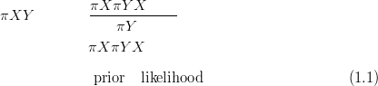
Unlike the classical approach, the Bayesian paradigm deals with all sources of uncertainty
in a coherent manner. The unknown statistical parameters X are treated as random
variables and a likelihood function π Y SX� is used to express the relative probabilities of
obtaining different values of this parameter when a particular dataset Y has been
observed. Prior probability densities πX� are placed on the unknown parameters
to reflect any subjective beliefs held before observation of data. The posterior
density πXSY � is delivered via Bayes theorem; it is a normalised product of the
prior and likelihood densities and reflects the updated beliefs in light of the
data.
Y SX� is used to express the relative probabilities of
obtaining different values of this parameter when a particular dataset Y has been
observed. Prior probability densities πX� are placed on the unknown parameters
to reflect any subjective beliefs held before observation of data. The posterior
density πXSY � is delivered via Bayes theorem; it is a normalised product of the
prior and likelihood densities and reflects the updated beliefs in light of the
data.
Bayes theorem constructs the posterior density πXSY � which is a summary of all
knowledge about the parameter X subsequent to observing Y . The posterior distribution
is a comprehensive inference statement about the model variables X. Any summary of the
posterior distribution is useful e.g. moments, quantiles, highest posterior regions and
credible intervals.
The Bayesian model presented in Haslett et al. (2006) is briefly described next. The
forward stage of the model infers the latent response of vegetation to climate given the
modern pollen counts and corresponding modern climate data. The inverse stage
then uses knowledge of the latent responses to infer climate from fossil counts
data.
Forward Problem
In this stage of the inference, the modern training data of pollen counts and
associated climatic data are used to inform probabilistic statements on the
unobservable response of vegetation to climate. The vectors of pollen counts at
each location are modelled as indirect observations of the unknown responses
to
the climate at that location. Building upon the notation already used in this section, the
responses are labeled X There is a vector of X responses at each point in the climate
space, one for each taxon. Each individual taxon then has a set of responses across the
climate space referred to as the taxon response surface; jointly over all taxa these are
denoted by X.
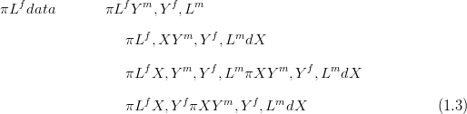
Bayes theorem is used as above to construct the posterior for the response surfaces
given the modern data, �Y m,Lm�.
 | (1.2) |
The integral in the denominator is typically not tractable analytically. In
Haslett et al. (2006) numerical integration was performed approximately using a
Metropolis-Hastings Markov Chain Monte Carlo algorithm.
Inverse Problem
The second stage of the Bayesian inference procedure is the calculation of posterior
probability distributions on the unknown palaeoclimates Lf, given the posterior for the
latent surfaces πXSY m,Lm� (derived in the first stage of the model) and the fossil pollen
counts Y f. This is the inverse problem (also known as multivariate non-linear calibration;
ter Braak discussion of Haslett et al. (2006)).
Sampled responses X are passed to an MCMC algorithm for sampling from the
posterior for palaeoclimate Lf given fossil pollen Y f and the surfaces X.
As the fossil pollen counts alone (without knowledge of the climate at which they
occurred) contribute little, or even no, information to the posterior for response surfaces
given data, πXSY m,Lm,Lf� is approximately equal to πXSY m,Lm�:
 | (1.4) |
The fully Bayesian approach is to solve the left-hand side of Equation (1.4); the
right-hand side is an approximation that is common to most inverse problems.
In fact, a positive feedback mechanism may occur if the fossil counts are
left in Equation (1.4); removing them may in fact lead to a more accurate fit.
This is referred to as “cutting feedback”; Rougier (2008) states that cutting
feedback, although technically a violation of coherence, may be presented in terms of
best-input. The model is trained using only the data about which the analyst is
confident.
Essentially, fitting the responses using the modern training data, for which counts and
climates are available, and
the fossil data, for which counts only are available, may lead to unwanted positive
feedback due to the fossil counts. The model training will begin by placing fossil counts in
a region of climate space; given this selected region, the response surface appears to fit
well. But the response surface was built using those counts in that region. The initial
choice has been strengthened, despite the fact that is was an arbitrary choice. Training
the model only on the modern data, for which climate is known, is preferred for this
reason.
Integration over the latent surfaces was via Monte Carlo integration in Haslett
et al. (2006): samples Xi,…,Xn are drawn from the posterior using the first stage
(forward problem) and passed to the second stage (inverse problem):
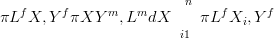 | (1.5) |
An alternative to MCMC for this task is proposed in this thesis. Namely, the suite of
approximation techniques referred to as INLA are applied and expanded for this purpose.
The implications of imposing any new modelling procedures and algorithms on the
forward stage are considered primarily in terms of the impact on the inverse
stage.
1.2 Computational Challenges
The most pressing challenges encountered in the Bayesian palaeoclimate project to date
involve the intensive computations necessary to carry out inference on the parameters of
interest. This is due mainly to an over-reliance on the computationally intensive Markov
Chain Monte Carlo algorithm. The large number of parameters required in the complex
modelling leads to serious concerns about the mixing the algorithm achieves in the
unknown parameter space. Linked to this is the problem that convergence is far
from assured, even after runs of the order of weeks (see Haslett et al. (2006)).
Additional detail in the model is prohibited due to memory and computation
concerns.
As discussed briefly in Section 1.1.1, the unobservable response surfaces must be
modelled non-parametrically. One way to achieve this is by discretising climate space on a
regular grid and modelling the response as a random variable at each node. High
resolution is desirable, requiring the use of a very fine discrete grid on the climate
variable space. This results in a very large number of latent variables. The paper
Haslett et al. (2006) dealt with a model including the order of 104 unknowns; and
this is for a inference performed on a greatly reduced dataset using a simplified
model.
1.3 Overview of Chapters
A brief outline of the research presented by chapter in this thesis follows.
Chapter 2: Literature Review and Statistical Methodology
A brief review of the literature on palaeoclimate reconstruction is presented. Progress
towards the standard set by Haslett et al. (2006) is charted and Bayesian statistical
methods for inverse inference are summarised. The remaining weaknesses in the current
methodology are outlined and the techniques used to overcome these in this thesis are
introduced.
Chapter 3: Models with Known Parameters
In order to separate modelling issues from issues of inference in the forward problem, this
chapter focusses on models with known parameters. Various model choices and the
implications of these choices are presented. Some new statistical models are detailed. The
novel contributions of this chapter are the methods for determining the decomposability
of large, multivariate models into separate, independent modules and the nested
compositional model. Issues related to the decomposition of models are introduced and
discussed.
Chapter 4: INLA Inference and Cross-Validation
The single biggest reduction of the computations required for a full Bayesian inference to
be performed on the palaeoclimate dataset are due to the approximation techniques
presented in this chapter. By approximating the posterior for the unknown variables in
the forward problem with a tractable multivariate density, Markov Chain Monte Carlo
may be avoided entirely. The posterior distribution for the responses may be
expressed analytically and thus issues regarding mixing and convergence are
avoided. The approximation error is typically lower than the Monte Carlo error
and the computations required are dramatically reduced. This allows for the
addition of extra detail to the model and dramatically increases the potential
of the application of the procedure to larger datasets, examples of which are
explored.
There are many modelling choices made throughout the application in Chapter 6.
These choices must be supported and alternatives explored. Cross validation is a useful
tool in evaluating the fit of the Bayesian models to the data. This is typically done by
computationally intensive Markov Chain Monte Carlo; it requires many repeated runs
and, for large problems such as the palaeoclimate reconstruction project, this may become
computationally overwhelming and is therefore not considered. Approximation methods
are once again discussed in this context along with further application to the pollen /
climate dataset.
Chapter 5: Inference Methodology
An investigation is carried out into the implications of decomposing the counts data
vectors and carrying out marginal inferences on each component of the vector
sequentially. This is at best identical to a joint inference on all components at once and at
worst an approximation to it. The accuracy of the approximation is expressed as a
function of several impacting factors and the conditions for exact reproduction of
the joint posterior from the marginal posteriors (perfect decomposition) are
described.
Details related to performing inference using the techniques already developed in
previous chapters are presented. This chapter serves as a platform towards the application
to real data in Chapter 6.
Chapter 6: Application: the Palaeoclimate Reconstruction Project
The motivating problem for the research conducted in this thesis is to improve and
advance the palaeoclimate reconstruction project. Therefore, a chapter is devoted to
applying the work developed in previous chapters to the RS10 pollen and climate dataset.
The various approximation algorithms allow for a richer modelling of the forward problem
(the response of vegetation to climate) than was previously possible. The modelling of
zero-inflation represents a fundamental change in the model. Practical issues regarding
the application of the new model and use of the approximations are identified and
discussed. Results are presented and compared with the results derived from previous
approaches. A fast cross-validation methodology for the inverse problem is central to this
chapter.
Chapter 7: Conclusions and Further Work
The results from the preceding chapters are summarised and discussed. An appraisal of
the work to date is conducted and outstanding issues and challenges are identified.
Solutions to these remaining challenges are suggested and alternative methodologies
briefly outlined.
1.4 Research Contributions
The following is a statement of the main contributions to the palaeoclimate
reconstruction project by the author as presented in this thesis:
- Investigation is conducted into the accuracy lost in sequential modelling of
individual plant taxa responses to climate.
- Nested compositional counts models for the palaeoclimate dataset are
introduced. It is demonstrated that knowledge of the nesting structure is
crucial to performing accurate inferences.
- A fast Bayesian inference procedure on the forward stage of the palaeoclimate
reconstruction model is demonstrated. This allows for far richer models to be
developed and, more importantly, validated.
- A model for parsimonious modelling of zero-inflation of the counts data that
is compatible with the INLA methodology is presented.
- A fast inverse cross-validation methodology using INLA is developed. This is
a novel extension to the technique and is demonstrated through application
to the pollen and climate dataset.