and a new count ynew.
This chapter deals with modelling issues as distinct from any challenges relating to statistical inference of latent fields and hyperparameters. In this chapter, model parameters are taken to be known and inference details for the forward problem are suppressed, to be dealt with in later chapters. Specifically, the forward stage of the model is taken to have all known parameters; inference on the inverse stage is used to assess different forward models.
The novel contributions contained in this chapter relate to model choice. Specifically, the following questions are addressed: Under what circumstances a large, multivariate model, such as those required for the motivating palaeoclimate problem, may be broken down to produce a series of independent, smaller and more manageable inferential tasks? How might one proceed with such a decomposition? How might the validity or accuracy of the decomposition assessed? Finally, when a model may not be decomposed directly, are there augmentations to the data that might facilitate decomposition?
When dealing with highly multivariate datasets, such as the RS10 pollen and climate dataset, several modelling choices present themselves. These consist of choices for modelling the latent parameters of the hierarchical model, the hyperparameters and the choice of likelihood model for the data given the parameters. It is necessary to make clear the motivations and justifications for each of these choices. This requires the use of “model fit” techniques. Cross validation is the tool selected in this work, the details of which are presented in Section 4.2.
Section 3.1 introduces the type of inverse problem investigated in this thesis for a single spatial process generating counts across locations.
Section 3.2 sets out the motivation for decomposing large, joint models into independent modules. A definition of decomposable models is given and conditions under which models may and may not be exactly disjoint-decomposed are presented. Finally, sources of interaction preventing decomposition are discussed.
A fully-Gaussian case in Section 3.3 allows for the introduction of several key modelling issues in a Normal context. The tractability and familiarity of the multivariate normal model are used to present modelling issues that apply in a wider context of multivariate modelling. Specifically, non-decomposable models are developed in the context of the multivariate normal model.
Departures from normality in Section 3.4 introduce additional issues related to counts data. Novel models for such data are also introduced in this latter section in the form of specialised likelihood functions, such as zero-inflated data models.
Section 3.5 deals with the constrained space associated with compositional data analysis. Some pitfalls of analysis on this space are described. Finally, novel models for specifying complex yet decomposable models for compositional data are presented.
Finally, conclusions are made from the work detailed in the preceding sections. These conclusions are carried forward into the later chapters.
Returning to the toy problem described in Section 2.5.2, a univariate process varies smoothly across a location space. That section demonstrated the effect of differing model hyperparameters on the inverse problem. The inverse predictive distributions were found to be multimodal due to the shape of the response surface. The shape of the response surface also influences the degree of accuracy to which the inverse problem (prediction of location given count) may be solved.
To recap, the goal is to infer unknown location l given training counts Ỹ with training
locations and a new count ynew.
As per Equation (2.24),
 | (3.1) |
A flat prior is used for π lnew�. The posterior for location l is therefore proportional to
the likelihood for count y at that location. The first task is to find πXSỸ,
lnew�. The posterior for location l is therefore proportional to
the likelihood for count y at that location. The first task is to find πXSỸ, �, the details
of which are suppressed in this chapter.
�, the details
of which are suppressed in this chapter.
In the following examples, the toy data comprises a single smooth response surface which generates univariate counts data. There is a single count at each of 10 sampling locations.
The immediate objective here is to identify the conditions for which inference in the inverse stage of the model is difficult. From the discussion above, the factors which influence the ability of the model to accurately predict climate given a new count and training data are the shape of the underlying surface and the prior and likelihood precision parameters (κ and 1sσY 2).
The performance of the inference will also be greatly effected by the new data presented to the model. Recall, for example, the multimodal posterior arising from the inverse stage inference given a new count of y2 � 252 in Figure 2.2: the inverse inference is placing large probability mass in another location; this must be classed as a poor inference and will occur (to varying degrees; see Figure 2.3) for any model parameters as it is due to the non-monotonic shape of the response function.
Conversely, given a new count of ỹnew � 450, the model will always place a unimodal inverse stage posterior on the very left of the location space; this is in fact the only area from which such a high count can have been generated, given the underlying surface. It is contrasting situations such as these that is the interest here; cross-validation and model fit are discussed in later chapters.
It is useful here to explore some interesting and challenging features of the inverse problem. The impact that the shape of the underlying latent response curve has on the posterior for location given count is demonstrated. Three examples are are presented in each of sections 3.1.1 and 3.1.2. Although both sections necessarily use examples given a new count, with unobserved location, Section 3.1.1 is new count value specific whereas Section 3.1.2 uses example response curves that will generate similar challenges regardless of the value of the new count.
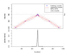
Loosely speaking, conditions may be subdivided into 3 categories; easy, medium and hard. These are due to encountering degrees of strongly informative data, weakly informative / uninformative data and misleading data respectively. These three categories are illustrated with examples in Figure 3.1 for fixed values of the model parameters, κ and σY 2.
The easy case refers to a problem that, due to the shape of the response function, delivers a tight, unimodal posterior distribution for the location (climate) given a count. The medium case delivers a diffuse posterior as the fitted response function carries little informtation on location given count. Finally, the hard case delivers a multimodal location posterior with the true location not necessarily located under the major mode. The posterior distribution for location may in fact place much probabilty mass far from the correct location, resulting in misleading predictions.
Figure 3.1(c) shows an important result; the performance statistic D (see Equation (2.32)) is not simply an indicator of the strength of the signal provided for the inverse stage but also of the uniqueness. Figure 3.1(c) carries a strong signal at the correct location, however the inverse stage posterior places higher mass at another, distant, location; this results in a poor performance rating.
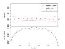
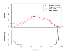
This is closer in spirit to cross-validation than the previous section. The goal here is to categorize training datasets based on the ability of the fitted model to predict locations given arbitrary new counts. Again, the categories are described as easy, medium and hard. Figure 3.2 depicts an example of each case.
|
Another cross-validation statistic that will be used throughout this thesis is the number of training data that fall outside the 95% highest posterior predictive distribution. The predictive distribution here is the leave-one-out cross-validation posterior predictive distribution for the location given all other locations and the counts data.
Definition 3 Δ is the % of data lying outside the 95% highest posterior density region of their inverse predictive density
If the model fits the data, then the expected value of Δ is 5%. This does not depend on the accuracy of the inverse predictions delivered. When the location space lies on a discrete grid it is not always possible to define a 95% HPD region. For a discretized space, the method for defining the 95% HPD regions is as follows:
This means that the HPD region contains 95% or more of the total probability mass. Therefore, the expected value of Δ is B 5%.
The concern in this thesis is the case of more than one response surface, each of which generates its own counts data. The simplest approach to the inverse problem is to perform inference on each set of counts separately for both the forward and inverse stage of the problem. The inverse predictive distribution given all components is then the product of all inverse predictive distributions for each of the components of the counts assemblage. Such a model, expressible as non-overlapping separable parts, is discussed in the next section.
Complex, highly multivariate datasets that require multivariate models pose several challenges of computation and model choice (see also Section 5.1). One approach in dealing with these challenges is to disjoint-decompose the problem into disjoint, independent modules. Each module requires a model to be fitted to a separate subset of the overall dataset and inference may be carried out separately on each subset, i.e. independently from the other subsets.
Definition 4 Multivariate models which may be expressed exactly as the product of disjoint parts are said to be disjoint-decomposable.
This is closely related to independence; a probability model that factorises into a number of (potentially multivariate) independent distributions, with no terms appearing in more than one distribution is disjoint-decomposable. There is no interaction between the margins of such models. However, many models that do not factorise in such a manner may be approximately disjoint-decomposable. This may allow for a far simpler inferential approach to be taken, with a post-hoc correction for the decomposition.
The difference between disjoint-decomposable and independence is subtle, but relevant in this work. If a model is comprised of independent modules then it is disjoint-decomposable. However, some models that are not expressible as the product of independent parts may decompose in practice.
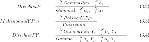
The simplest example of this is with regard to compositional data. If counts proportions data Y with sum n are modelled with a Multinomial distribution then it is immediately clear that the data are dependent. However, the data may be modelled as independent Poisson counts and the product of the marginal likelihoods then gives an approximation to the true, joint likelihood. The approximation error can be corrected by dividing by the probability that the total count is n. This probability is available trivially as a Poisson count.
If inference on the parameters P of the Multinomial are modelled with a Dirichlet prior then the posterior is Dirichlet. Decomposing the model into independent Poisson likelihoods with independent Gamma priors yields a product of Gammas as the decomposed-model posterior. To correct the approximation error this product is then divided by the posterior distribution on the sum.
So, given a counts vector Y , constrained to sum to n with a Dirichlet prior with parameters α and a Multinomial likelihood, the Dirichlet posterior may be written as a product of Gammas, scaled by a Gamma distribution on the sum:
If the model does not disjoint-decompose then the model corresponding to a decomposable version approximates the joint model. Inference on such a model will approximate joint inference on the non-decomposable model. This is dealt with in Chapter 5. The accuracy of the approximation of the decomposable model to a non-decomposable version depends on the level of interaction between the modules. Simple performance checks such as the one described in Section 3.2.2 may be used to determine the legitimacy of decomposing the model.
If the model does not decompose into univariate marginals, decomposition into smaller, more manageable multivariate marginals may still render the inference to be far simpler.
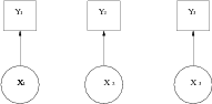
A simple and intuitive decomposition of the pollen dataset is by taxon (plant type). Under this model, each taxon response is modelled as conditionally independent, given the climate. The problem described in Section 3.1 is for a single response surface. The predictive distribution for climate is computed given the count for this single taxon. Repeating the inference procedure separately for each taxon marginally and taking the product of the climate predictive distributions yields a predictive probability distribution over all taxa, given the vector of taxa counts. A simple graph of such models is shown in Figure 3.3.
|
|
The marginal inference on each taxon, independently of the others, allows for many conveniences for the computational inference (discussed in Chapter 5) and in model design. As there are only a handful of hyperparameters associated with modelling each taxon and a single latent surface, both the model and the inference are simple. Interaction between taxa is not allowed in the marginal model so modelling interactions do not have to be considered.
The following section describes a method for testing the validity of the conditional independence assumption that is required to disjoint-decompose the model.
If marginals / decomposable models are used erroneously, errors are incurred. The error increases with the number of dependent parts that are modelled independently.
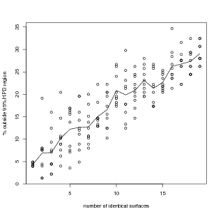
Figure 3.4 demonstrates how, for toy data, a cross-validation error statistic increases with each additional component modelled. Each entry in a vector of observations occurring at multiple locations in a uni-dimensional space is modelled as an indirect observation of a latent parameter. These latent parameters vary smoothly across the location space and are modelled as GMRFs, independent of the other latent surfaces.
The data are generated from a latent field composed of 15 identical smooth surfaces defined on a regular grid of the location space. These surfaces are not independent given the locations, however they are modelled as such in order to facilitate decomposition of the problem. This induces the errors, manifested in the plot as an increase in the percentage of points falling outside their corresponding leave-one-out predictive distribution’s 95% highest posterior density estimate with each surface added. This is the cross-validation Δ statistic introduced in Section 3.1 and has an expected value of less than or equal to 5%.
|
|
Such dependence can occur as a result of direct interaction or through the joint dependence on unobserved covariates. If the model needs to incorporate dependency between these multiple surfaces, an overall covariance model must be set up. This is most readily discussed in the Gaussian context of the following section.
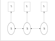
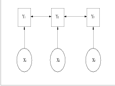
These interactions may be modelled as either non-zero precision terms in the multivariate prior or in the likelihood. Figure 3.5 shows graphs for these two models.
|
If a joint model is not decomposable, there must be non-zero off diagonal terms in either the prior or the likelihood precision matrix corresponding to inter-taxa dependence. It is the source of interaction that determines where these non-zero terms should occur. For multivariate Bayesian hierarchical models, such as the motivating palaeoclimate reconstruction problem, the following potential sources of interaction across plant taxa are identified. Each source may prevent model decomposition.
Additional, covariate information Z is sometimes available for large, multivariate datasets. For example, in the RS10 pollen and climate dataset, altitude, longitude and latitude are available. If, given climate, the propensity to produce pollen is thought to depend on one or more of these covariates then the response surfaces will not be independent.
A common approach to including this in the modelling is to model the counts data as dependent on the response surface values plus the covariate data times a vector of unknown regression parameters β.
 | (3.5) |
If the data are conditionally independent given locations (climates) and covariates, then they should not be modelled as conditionally independent given the locations only. In this case, the interaction occurs indirectly through the covariates.
Interaction at the data level may occur as a result of direct competition. Interactions of this type are independent of the underlying response and should therefore be modelled in the likelihood precision matrix. An example in terms of the motivating pollen dataset would be competition for resources between plant types.
The data collection mechanism may produce non-zero correlation between otherwise independent components of the data. For example, if the data were collected until a preset total were reached, then this would not only set an upper limit on the counts data; a negative correlation between the entries of the data vector would also be produced, due to the sum-to-total constraint.
Since the information carried by the data now resides in the relative proportions, rather than absolute values, the model should be for these proportions. Therefore, a sum-to-unity constraint must apply to the latent parameters. For example, if the data likelihood model were Multinomial, then an appropriate distribution on the parameters of the Multinomial would be defined on the simplex (Section 3.5.1).
However, an important observation that was was missed in Haslett et al. (2006) is that such models may still be disjoint-decomposed, provided the data are in fact conditionally independent given the constraint. This is discussed in some detail in Section 3.5.7.
If the data are modelled as Gaussian given Gaussian latent parameters then inversion of the model may be done analytically. Although the data of the motivating problem are integers (counts data) and thus are not suitably modelled as Gaussian, the familiar Gaussian framework does allow for some of the modelling nuances dealt with in this chapter to be introduced in an easily demonstrated context.
Furthermore, the inference procedure introduced in Section 4.1 is directly motivated by and related to the Gaussian model. Therefore, lessons learned from the multivariate normal model can be readily applied to a more general context of inference.
Constructing non-decomposable probability models requires explicit modelling of the covariance between interacting modules. Again, the familiar Gaussian context is useful to illustrate some important aspects of such models.
There are various models for multiple response surfaces that do not disjoint-decompose as the product of their marginals. These involve models for which there are various forms of interaction, either between the counts data, given the responses, or between the responses themselves, given the locations. This is manifested in the model as non-decomposable multivariate joint likelihoods or non-decomposable multivariate joint priors, respectively.
It is very important to again note that even if such interactions exist, but are not built into the joint model, then the model will still disjoint-decompose. Inference will be identical, albeit flawed, for the joint model and the product of the by-taxon marginals.
If interaction (dependence) is to be modelled, it arises in the Gaussian context either in the latent parameters precision matrix or in the likelihood precision matrix. In either case, the relevant precision matrix will have non-zero entries for between components (taxa) interactions. Note that in all cases considered, there are non-diagonal terms in the prior precision matrix for each taxon. These are intra-taxon terms and are a result of the prior belief on the smoothness across location space of the latent responses. Thus, for a model with multiple non-interacting / independent taxa, the overall precision matrix is block-diagonal. Each block is then the (independent) taxon-specific precision matrix.
This is best illustrated by means of a very simple example. Suppose there are two counts Y at each of two locations in a 1D location space L ��l1,l2�. This gives a total of four counts Y ��y11,y12,y21,y22�, where the subscript indexes the components of the counts vector and the superscript indexes the location. i.e. yij is the count for the ith component at the jth location.
The model requires four latent variables X ��x11,x12,x21,x22�, using the same indexing as for the data. The fully Gaussian hierarchical model is then specified entirely by the following multivariate normal distributions:
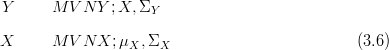
Specification of the full, joint model now involves specifying the hyperparameters �μX,QX� and the likelihood precision matrix QY .
The posterior distribution for X is also multivariate normal with mean and precision matrix given by
If either QX or QY have non-zero terms for precisionx1,x2� or precisiony1,y2�
respectively, then the posterior precision matrix Q will also carry these non-zero terms.
Therefore, the posterior will not disjoint-decompose exactly and the product of posterior
marginals will not equal the full joint posterior.
It is worth reiterating at this point that if both the prior and likelihood disjoint-decompose, then so does the posterior. This is easily seen in the context of the multivariate normal as if both terms on the right hand side of Equation (3.8) do not contain non-zero terms preventing decomposition, then their sum, giving the posterior precision matrix, will also not contain such terms. Hence, the product of (perhaps multivariate) marginals will yield exactly the joint posterior and the model thus disjoint-decomposes.
If a model with inter-surface interactions is required then there are four options. Specification is through one of:
The first two options are closely related in the context of multivariate normal models for both the prior and the likelihood. Which of these two to incorporate depend on the model and are problem specific. The source of interaction informs the choice of modelling interaction in the prior or in the likelihood. The last two options involve inference issues and are dealt with in Chapter 5.
The precision, or “degree of mutual agreement”, of xi1j1 and xi 2j2 is
 | (3.9) |
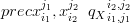
As this is a four dimensional indexing, it is necessary to construct a system for
indexing across both surfaces / counts and the location space using a single index to yield
a two dimensional precision matrix. The convention adopted here is that the subscript i
and superscript j pairing becomes single index i� 1�NL �j, where NL is the total
number of discrete points in the location space. Note that there is one surface per taxon
for the pollen data example.
The overall precision matrix covering all possible (process, location) pairings for the latent parameters X is then:
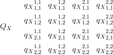 | (3.10) |
Rows of QX denote the precisions for individual surfaces across locations and columns denote inter-surface precisions at a point in the location space. If the latent surfaces are modelled as conditionally independent, given location, then qXi1,j1i2,j2 � 0 for i1 ( i2, regardless of j1 and j2.
qi1�i2 are intra-surface parameters and may be reduced to a single hyperparameter via imposition of a regular structure as shown in Section 2.2.4.
Interaction between surfaces is modelled as being a local effect in the location space. i.e. precision, for a common location, between two surfaces is the same across the locations space. Interaction between surfaces at non-equal locations is modelled as zero. Consideration of whether the joint model disjoint-decomposes exactly now amounts to checking whether the posterior precision matrix is block-diagonal. (Diagonal implies total independence; block diagonality is a consequence of the conditional independence across taxa, but not across climate; see Section 3.2.1.)
The data are typically modelled in Bayesian hierarchical models as being conditionally independent, given the level two parameters. This implies diagonal precision and covariance matrices QY and ΣY . If interaction between components is at the data level, then this is no longer the case.
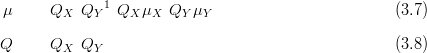
However, for the model with multivariate normal likelihood with multivariate normal prior, the multivariate normal posterior will have the exact same precision matrix whether the interactions are placed in the likelihood precision matrix or the prior precision matrix as it is simply a sum of the two. The posterior mean will be slightly different; however it is simple to show that for any choice of inter-surface precision parameters in the likelihood, there exists a set of inter-surface parameters for the prior precision matrix that yield the same posterior mean.
In the following the notation is that the model with interactions in the likelihood precision matrix is given the superscript A and the model with the interactions in the prior takes the superscript B. If the prior is zero-mean and the posterior means under each model are taken to be equal:
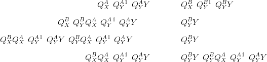
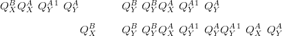
The above demonstrates the similarity between modelling interaction at the prior and at the likelihood precision matrices.
Errors are incurred if a decomposable model is applied to data that have arisen from a
model that does not disjoint-decompose. In the context of this section (Normal models
with known parameters), this arises as setting the multivariate likelihood precision matrix
terms that relate to between-module interactions to zero. If Q is the true, joint precision
matrix, then  is the disjoint-decomposed model precision matrix with all interaction
terms set to zero. If the model disjoint-decomposes, these two matrices will be
identical. If not, the disjoint-decomposed model will be an approximation to
the true model. The accuracy of this approximation will of course depend on
the level of interaction between the modules that are treated as independent
in the disjoint-decomposed model. A toy model demonstrates this as follows:
is the disjoint-decomposed model precision matrix with all interaction
terms set to zero. If the model disjoint-decomposes, these two matrices will be
identical. If not, the disjoint-decomposed model will be an approximation to
the true model. The accuracy of this approximation will of course depend on
the level of interaction between the modules that are treated as independent
in the disjoint-decomposed model. A toy model demonstrates this as follows:
suppose “counts” data are generated a multivariate normal distribution with mean μ and
precision matrix Q
 | (3.11) |
where the length of μ is the product of the number of discrete locations NL and the number of surfaces NT . These surfaces vary smoothly across locations so that given a new vector of counts, the model may be inverted and the location associated with these counts predicted. In this example, NT � 2 and NL � 10.
Using the same indexing system in Equation (3.10) to index over components and locations, the full precision matrix for two components in two locations will be decomposable as the product of marginals iff qi1,j1i2,j2 � 0 for all i1 ( i2. This equates to whether Q is in fact block-diagonal, with the number of blocks equal to the length of the data vector at each location NT and the length of the side of each square block equal to the number of discrete locations NL.
Provided interactions between counts are consistent throughout the location space, symmetric, and that there is no interaction between data at disparate locations, then there are �NT 2 � interaction terms. Thus, for two such surfaces, there is a single parameter ρ governing interactions.
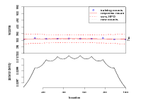
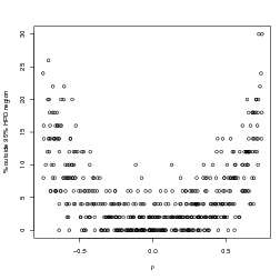
Intuitively, the closer this parameter is to zero, the closer Q is to being block-diagonal and thus the closer the joint model is to being decomposable. Replications of the above toy model, for varying values of ρ, the scalar interaction parameter, show this relationship empirically; see Figure 3.6. For each replication, two new randomly generated smooth response surfaces are generated; thus the results in the figure are generalised across all shapes of response surface. The counts data at location j come from random draw of a bivariate-Normal distribution with mean equal to the two responses at that point and precision matrix given by
 | (3.12) |
It can be seen from Figure 3.6 that the greater the absolute value of the interaction parameters ρ, the more points fall outside their 95% HPD region for the inverse predictive distribution. The mean of the percentage outside the 95% HPD region is less than 5% at ρ � 0 due to the use of discrete HPD regions. Only regions of 95% or more may be specified so that the percentage outside is expected to be 5% or less. Section 5.3.1 discusses this in more detail.
|
|
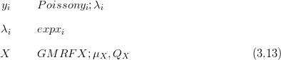
Non-Gaussian likelihood models are introduced and examined in this section. This leads to posteriors that are typically not available in closed form. The main concern is with multivariate counts data; treated as conditionally independently using models such as the Poisson and various related distributions or with multivariate counts likelihoods for the case of vectors of constrained counts data. Section 4.1 will show how closed forms for the posterior will be achieved for these non-Gaussian likelihoods and Gaussian priors.
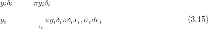
For all models that disjoint-decompose, each element of a constrained counts vector is modelled independently of the rest. In the simplest case for counts data, the counts are modelled as being Poisson distributed, with the rate parameter derived as a deterministic function of the underlying latent surface. Thus, for the hierarchical model, with log-link for the rate parameter and a GMRF prior
If the “effort” spent on counting the data varies across the sampling space, then this will effect the expected and observed counts. A more general form of the Poisson distribution with an additional “effort” parameter allows direct modelling of this effect. For example, if the time t spent collecting counts data Y were to vary, then the scaled Poisson distribution for those counts, with rate λ would be
 | (3.14) |
For the motivating pollen dataset, the time or effort spent in counting the data is unknown; what is available is the total count across all plant taxa. This can be used as an observed surrogate, or proxy, for the effort / time spent collecting the counts for each taxon. In fact, this total count imposes a constraint in the form of a strict upper limit on the count for each individual taxon. Counts thus constrained are typically modelled using the Binomial distribution, or a related distribution.
Of particular interest here is data for which there is overdispersion; i.e. the single rate parameter of the Poisson distribution is insufficient as the variance is greater than the mean of the data, given the parameters. Zero-mean, normally distributed non-spatial random effects may be added to the parameters, resulting in overdispersion with respect to the spatial component of the latent surface.
The data are then indirect observations of a latent variable with two distinct parts; a spatially structured part X and a random effects part ϵ.
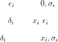
This results in double the number of latent random variables in the model and at least one extra hyperparameter (the variance of the random effects), which is an undesirable situation. An alternative is to introduce random effects that are modelled using a distribution that is conjugate to the likelihood. The random effects may then be analytically integrate out, leaving a reparameterised, closed form likelihood that has a variance that is larger than the mean.
For example, the data Y is Poisson given the rates λ; the rates are a mixture of a spatially smooth part X, modelled as a GMRF, and a non-spatial random effect δ. If this zero-mean random effect component is such that the product of the spatial part and the random effect is Gamma distributed, with mean equal to the spatial part, then the hierarchical model is:
This counts distribution carries just a single extra parameter (δ) over the simple Poisson model. δ controls the degree of overdispersion.
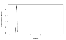
If a non-zero inflated likelihood is used for data that are zero-inflated, then inference on the parameters of that likelihood will be erroneous. Specifically, the extra zeros will reduce the unobserved mean parameter of the likelihood and will increase the variance. In the context of this Chapter (models with known parameters), the inverse predictive distributions will misplace probability mass if inversion is done using the wrong (i.e. non-zero-inflated) likelihood function.
This will occur in a predictable manner; the non-zero-inflated model will place inverse predictive probability mass for zero counts exclusively at the regions for which the response function is lowest. Non-zero counts will be treated the same as for an equivalent zero-inflated likelihood and will therefore be correct. The degree of zero-inflation will thus govern the degree of the error of the non-zero-inflated model when applied to zero-inflated data to generate inverse predictive distributions.
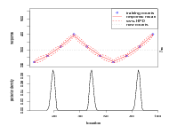
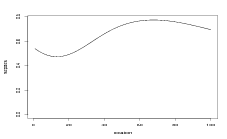
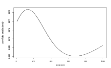
A toy problem example is once again employed to illustrate this point. A smooth surface p in a uni-dimensional discrete space gives the (known) parameters for a zero-inflated Binomial likelihood:
 | (3.18) |
where q � pα, α � 0.3
and n � 1000 is the total count.
Results for the inverse predictive distribution given known, deterministic forward models are shown in Figure 3.7. The result of applying a non-zero-inflated model to zero-inflated data is clearly demonstrated; under the non-zero-inflated model, all zero-counts are inferred to arise exclusively at the lowest points of the response curve. This is because the non-zero-inflated model will generate most zeros in this are of the locations space. While the zero-inflated model still necessarily reconstructs the same location of least response as being most probable, the curve is not nearly so peaked. This, being the model from which data was simulated, gives the correct predictive distribution.
|
|
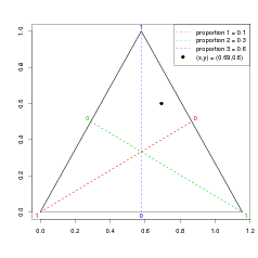
If a vector p ��p1,…,pN� has all non-negative elements representing proportions of a whole then the vector is constrained to sum to unity
 | (3.19) |
Such vectors of proportions are compositional data and are frequently and erroneously modelled using techniques developed for unconstrained spaces (Aitchison (1986); Aitchison and Egozcue (2005)).
Due to the constraint, the data have one less degree of freedom than the length of the compositional vector. The full vector may be completely specified using the components of any N � 1 subvector (the left out value being determined as one minus the sum of the subcomposition). Any such subvector completely specifies the full composition.
The set of all possible vectors for a given length of composition is referred to as the simplex space . The simplex space for a compositional vector of length N with unit-sum constraint is then N � 1 dimensional.
|
|
There are two contrasting approaches to modelling compositional data in a coherent manner that do not fall into the trap of using traditional, unconstrained multivariate statistics:
These two competing approaches require different models to be developed. The latter typically uses multivariate normal distributions and established Gaussian theory; this leaves choice of transformation and subvector as the main decisions to be made in the modelling sense. The former requires alternative distributions, defined directly on the simplex space.
Although progress has been made on statistics defined on the simplex space, the availability of a rich and established theory of multivariate analysis makes the use of the transformation technique the more appealing option. This is the approach advocated by Aitchison (1986) and is more widely adopted. In fact, distributions defined on the simplex space tend to have strong implied independence structures.
The majority of distributions defined on the simplex sample space are of the Dirichlet class. Despite the sum-to-one constraint, this class has an inflexible covariance structure making it unsuitable for many applications. The Dirichlet is the multivariate generalisation of the Beta distribution with probability density given by
 | (3.20) |
Although all N elements of the compositional vector p appear in the density calculation, the distribution itself is defined on the N � 1 dimensional simplex as pi is uniquely determined by p�i. η are the parameters of the Dirichlet distribution.
The covariance between two components of a Dirichlet distributed compositional vector is
 | (3.21) |
for i ( j. Thus, for modelling positive covariances between components, the Dirichlet distribution is entirely unsuitable. The covariance structure in the Dirichlet is entirely due to the sum-to-one constraint; this is why the Dirichlet is said to have a strong implied independence structure. Given the constraint, the components are necessarily modelled as conditionally independent.
A Dirichlet with parameter vector η may be expressed as a product of Gamma distributions, with shape parameters η and rate parameters all equal to Piηi, conditioned on the sum = 1 following a Gamma distribution with shape and rate both equal to Piηi.
 | (3.22) |
If sampling from the Dirichlet is required, this can be achieved by sampling from the Gamma marginals and then rescaling such that the sum is one. In fact, this is the usual algorithm for sampling from a Dirichlet distribution.
The Generalized Dirichlet distribution (Connor and Mosimann (1969)) has a more general covariance structure, achieved by doubling the number of parameters. If the number of components is N, then a Generalized Dirichlet (GD) distribution has two sets of parameters, each of length N:
 | (3.23) |
In the Generalized Dirichlet distribution, one of the components is always negatively
correlated with the rest. The other components may be positively or negatively correlated
with each other (Wong (1998)). Labelling the component that is strictly negatively
correlated with the rest as p1, if i,j A 1 then covpi,pj� may be positive or negative.
However, for any index greater than the lower of i,j, the sign of the correlation will stay
the same. i.e. :
One class of distributions on the N dimensional simplex that have a richer covariance structure than those provided by the Dirichlet class of distributions is defined by distributions in an unconstrained multivariate space (e.g. ℜN) with transformation to the simplex space.
This is the approach advocated and developed by Aitchison (1986). The proportions are transformed to the real space through the use of a transformation function. Standard multivariate analysis is carried out on these transformed variables (typically using multivariate Gaussian distributions) and the results are transformed back to the simplex space using the inverse of the original transforming function.
If N dimensional multivariate normally distributed real random vectors are transformed to the simplex space in N dimensions using the one-to-one inverse centered logratio transform:
 | (3.25) |
then the compositional vectors on the simplex are said to have a centered Logistic-Normal distribution (Aitchison (1986), Aitchison and Egozcue (2005)). The transformation from the simplex space to the real space is the centered logratio transform is given by
 | (3.26) |
the second term being there to centre the real vector around zero. There are other, closely related transformations that give rise to similar distributions (such as the additive Logistic-Normal). The general term for such distributions is Logistic-Normal and the centered Logistic-Normal is the distribution used in this thesis.
The advantage of transforming to the real space is that standard multivariate statistical procedures and models based on the multivariate normal distribution are made available. This allows for rich, well developed models to be used for the real-space X parameters, before simply transforming back to the simplex space.
Arbitrarily rich covariance structures may be built for the compositional vector through specification of multivariate normal distributions on the real space. The entire battery of existing techniques for the Normal distribution may be employed.
Chapter 6 of Aitchison (1986), shows that for any Dirichlet distribution with parameters δ large enough that probability mass is highest at the centre of the simplex then there is a very close Logistic-Normal distribution with diagonal covariance / precision matrix.
The approach broadly used in this thesis is to define normal priors on an unconstrained space with transformation to the simplex. The motivation for this is not in fact in the conveniences arising in the Normality assumptions across the composition, but because modelling latent surfaces as Gaussian and Markov across the location space allows for the use of the specialist multivariate inference techniques introduced in Section 2.2 and detailed in Chapter 4.1.
Extra unknown parameters could be introduced to model the inter-dependence, but this is an inference question and is therefore dealt with in Chapter 4.1.
Interest in this thesis is in models with some inter-process covariances that do not require either of the following:
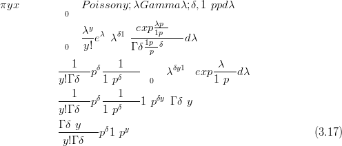
Although the Multinomial is a multivariate likelihood, with known covariances between components, it can be expressed as a product of independent Poisson distributions, with parameters equal to n�P, conditioned on the sum being equal to the total count n. This sum (Piyi � n) itself follows a Poisson distribution with rate parameter n.
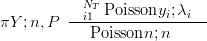 | (3.27) |
with λi � n � pi and Poissonyi;λi��
Thus, if a model using a decomposable likelihood function (such as the Multinomial) and a prior with conditional independence (such as the Dirichlet or indeed an Aitchison type prior with no inter-component covariance terms) is employed, then the posterior has conditionally independent components.
For the multivariate normal model, the prior and likelihood precision matrices in this case will be block-diagonal with no inter-component entries being non-zero. Thus, the posterior precision matrix, which is the sum of the prior and likelihood precision matrices, is also block-diagonal. The joint model, which is multivariate normal is therefore equal to a product of smaller multivariate normals, each describing a separate component of the composition. Thus, the model disjoint-decomposes exactly.
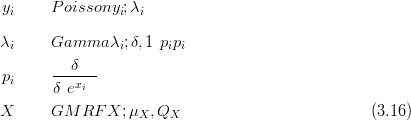
For constrained, multivariate counts data, the simplest example is of a Dirichlet prior with a Multinomial likelihood. Due to conjugacy, the posterior for the latent parameters is also Dirichlet. Inference on these parameters may therefore be carried out on each component separately and the joint distribution may be constructed from the marginals post-hoc by conditioning on the sum.
In the paper Haslett et al. (2006), the Multinomial was mixed with a Dirichlet distribution and a compound-Multinomial (or Dirichlet-Multinomial) distribution was formed for the likelihood. Although overdispersed with respect to the Multinomial, this distribution still enforces the conditional independence assumption.
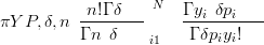 | (3.28) |
where n is the total count, δ is a scalar overdispersion parameter, N is the number of components of the composition, Y are the counts and P are the parameters of the Multinomial.
The derivation of this likelihood is as follows, starting with the mixing of a Multinomial with a Dirichlet with parameters δP:
 | (3.30) |
The integral is over a valid probability distribution and is therefore equal to one, yielding Equation (3.28).
Section 3.5.2 shows how common Dirichlet class distributions on the simplex have a strong implied conditional independence structure. Section 3.5.5 shows how multivariate, constrained likelihood functions such as the Multinomial may be disjoint-decomposed. The Generalized Dirichlet described in Section 3.5.3 allows for the breaking of this independence structure. However, it has double the number of parameters and still only allows for positive correlation between one component with all the others.
Aitchison type models, using a transformation from unconstrained, multivariate normally distributed, vectors in the unconstrained space to the simplex space provide an extremely rich class of model. However, they require either a prior knowledge of all interaction parameters or a specification through a large array of hyperparameters.
The former is unsuited to the pollen dataset; there is no such prior knowledge and interactions between components of the data vectors (whether through actual interaction or due to joint dependence on unobserved covariates) should be modelled in the likelihood.
The latter leads to problems of inference; specifically, the inference method of Section 4.1 requires a low number of hyperparameters and the conditional independence of the data, given the parameters (latent random variables).
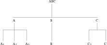
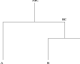
Nested models provide an interesting alternative; these are models in which there is more than one “level”. 1 This is graphically illustrated in Figure 3.9. Each level itself comprises a composition; each component of the composition may then be split into another composition on another level. The structure of the nesting refers to the number of levels and the splitting of each component into sub-compositions at each level.
|
|
A big advantage of such models is that they are still independent (given the constraint) at each level, provided the nesting structure is known. Unconditionally, the lowest level may exhibit a richer correlation structure than is possible with a Dirichlet model.
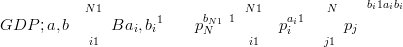
In Figure 3.9, for a Multinomial nesting, the total count is A � B � C; level 1 is a Multinomial of length 3 with components �A,B,C� and parameters �PA,PB,PC�, with PA �PB �PC � 1. A is further split into 3 components on level 2 and these are also Multinomial with total count A and parameters �PA1,PA2,PA3�. C is Binomial (Multinomial of length 2) at the second level, with total count C and parameter(s) PC1 (PC2 � 1 � PC1). It is easy to show that the lowest level is then also Multinomial, with parameters �PAPA1,PAPA2,PAPA3,PB,PCPC1,PCPC2� and total count A � B � C.
These two models then yield the same joint likelihood; i.e. a nested Multinomial is equivalent to a Multinomial on just the lowest level of each nest. Thus, knowledge of an existing nesting structure does not change the likelihood, if all nests are modelled as Multinomial.
For a nested Dirichlet model, the lowest level is not expressible as a Dirichlet. Isoprobability contours are a useful tool in illustrating the types of correlation structure achievable through various distributions. On the simplex, they demonstrate that, regardless of the parameters, the Dirichlet has strictly convex contours, due to the implied independence structure (Wong (1998)). The nested Dirichlet, however, can give rise to concave contours, showing positive correlations between components.
In the case of building priors for compositions, Wong (1998) shows that the Generalized Dirichlet allows for a more general covariance structure. Examination of the algorithm used to generate samples from the Generalized Dirichlet reveals an interesting result; the Generalized Dirichlet may be thought of as a series of two component nests. Indeed, Tian et al. (2003) touch on this briefly, noting that the nested Dirichlet is a special case of the Generalized Dirichlet.
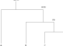
However, this is strictly for the case of a nesting structure composed of nests of size 2 only; i.e. nested Betas (see Figure 3.10). This is most clearly seen by examination of the sampling algorithm for the Generalized Dirichlet (as per Wong (1998)):
|
|
Thus Wong (1998) shows how constructing a prior, given knowledge of this nesting structure with binary splitting, gives rise to a Generalized Dirichlet for the lowest level with the b parameters weighted by the number of splits to each component.
A more general nesting structure, such as that shown in Figure 3.9 cannot be written as a Generalized Dirichlet; however, it can be written as simply the product of the Dirichlet distributions at each nest. Thus constructing a prior with knowledge of the nesting structure is straightforward. A rich covariance structure for the lowest level is obtained, with the covariances entirely dictated by the nesting structure.
|
|
The comparison between the prior for the nested model and the equivalent non-nested model is pleasantly straightforward. For the simplest case, shown in Figure 3.11, the nested model has Dirichlet prior for the first level:
 | (3.32) |
the prior being centred on �1s3,2s3�, since knowledge of the nesting structure dictates that BC must ultimately become two parts. The prior precision is dictated by the single δ parameter.
Similarly, the second level has Dirichlet prior:
 | (3.33) |
The product of Equations (3.32) and (3.33) gives the nested model prior.
The model without knowledge of the nesting structure has prior equal to
 | (3.34) |
Therefore the ratio of nested model to non-nested model is proportional to
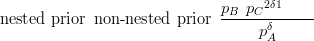 | (3.35) |
The interpretation of this simple ratio is that the nested model has a more flattened out probability distribution on the simplex. Greater variability has been achieved by recognizing that ABC does not split directly into three components, but undergoes two binary splits. More generally, the ratio will be proportional to a fraction with numerator equal to the product of intermediate priors. The denominator is a correction term for the weightings given to each component of an asymmetric split.
In fact this is problem specific, as some models will be constructed giving equal a-priori probability to A and BC in the above example. In this case, the result is the same but with no term below the line in Equation (3.35).
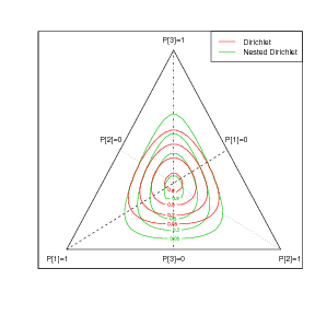
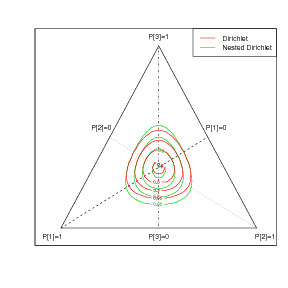
For unbiased priors (no knowledge of the nesting structure), this results in asymmetric priors on the simplex that are nonetheless centred about the middle of the simplex (see Figure 3.12). In this case, the isoprobability contours are a-priori convex. However, the posterior may be part concave, unlike the restrictive Dirichlet posterior obtained from a Dirichlet prior and Multinomial likelihood.
|
|
In the case of a Dirichlet prior and Multinomial likelihood for each nest, the comparison between the posterior for the nested model and the equivalent non-nested model is similar to the Dirichlet prior case of the previous subsection. The posterior is Dirichlet (due to conjugacy between the Dirichlet priors and Multinomial likelihoods at each nest). Therefore, the ratio between the nested model posterior and the non-nested posterior is similar to Equation (3.35) and is given by:
 | (3.36) |
where yi is the count associated with component i.
|
|
For an overdispersed compound-Multinomial model for the counts, the algebra is not as neat for the ratio of nested to non-nested models. The posterior for a Dirichlet prior and a Multinomial likelihood provide a guideline; the overdispersed compound-Multinomial model for the counts is equivalent to an integral over auxiliary compositional parameters and is therefore an average of such models. The following section shows empirical results for the comparison between nested and non-nested compound-Multinomials in terms of the inverse predictive power when the data are indeed generated from a nested compound-Multinomial likelihood.
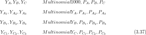
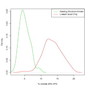
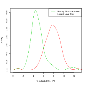
A simple toy problem using data simulated from a known model illustrates the impact of a nesting structure. At regular locations in a 15 � 15 grid, 3 counts are distributed according to a Multinomial distribution of length 3. The 3 parameters of this distribution arise from a Dirichlet mixture of length 3 of a transformation to the simplex space of stochastically smooth fields X (i.e. the likelihood is compound-Multinomial). Each of these 3 counts is subdivided into 3 more counts; again according to a compound-Multinomial distribution.
Therefore, at each location in the 2 � D regular lattice:
with all P parameter vectors being Dirichlet mixtures of corresponding compositional vectors ϕ.
 | (3.38) |
where δ is a scalar controlling the degree of overdispersion.
The vectors ϕ vary smoothly across the location space and the sum-to-unity constraint applies everywhere and at both levels.
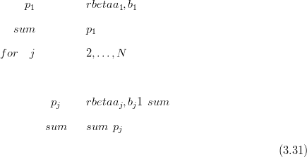
The Dirichlet mixtures are proportional to Li�13piδi�1 where δi � δϕi. The Multinomial part is proportional to Li�13piyi. The compound-Multinomial is the product of these two and is therefore proportional to Li�13piδi�yi.
The full, joint density of the compositional vector at each level is proportional to the product of the 3 lower level compound-Multinomials times the compound-Multinomial for the first level. The non-nested model differs only due to the overdispersion (the likelihood for a nested Multinomial is itself a Multinomial; Section 3.5.6).
Comparison of Figures 3.14 and 3.15 show this result. In both cases, a look at the number of cases generated from the nested model that fall outside the corresponding 95% HPD region for the inverse predictive distribution under the non-nested model is greater than it should be. However, the error is less for a larger overdispersion parameter, corresponding to a lower extra, non-spatial variability. i.e. more overdispersion leads to higher incurred error when nesting is ignored.
|
|
|
|
Inference using large, compositional models may be difficult or even impossible due to computation and memory constraints, or compatibility issues with inference techniques (see Chapter 4). In these circumstances, approximating the joint model with a decomposable model might provide more accurate results than attempting to use the non-decomposable model.
Although compositional models may appear to be inherently non-decomposable, they do disjoint-decompose provided the modules they are to be disjoint-decomposed into are conditionally independent, given the constraint. For example, given a Multinomial likelihood and a Dirichlet prior, the Dirichlet posterior may be expressed as a product of independent Gamma distributions divided by a Gamma distribution on the sum. Inference for the forward stage of the model may then take place in the unconstrained space with response surfaces fitted to the counts individually. The joint model is then constructed by conditioning on the probability of the sum being equal to unity. The distribution on the sum is a single, straightforward calculation.
An important detail to note here is that the joint problem has been disjoint-decomposed into the product of the unconstrained marginals. The product of the constrained marginals (Betas for the Dirichlet and Binomials for the Multinomial) do not give the correct joint model.
For the inverse predictive stage, given the fitted forward model, the inference cannot be disjoint-decomposed. However, this is typically a far smaller calculation and so can be done using the non-disjoint-decomposed joint model. Inversion of the model amounts to integrating out the latent parameters of the model at each point in the location space to yield the marginal likelihoods at each point.
If the forward stage yields closed form posteriors (as is always the case in this thesis; see Section 4.1), then simple Monte-Carlo integration for the multidimensional integral required for the sum delivers the required distribution. If the forward stage posteriors can only be sampled from (e.g. via MCMC), then MCMC may be used again for the inverse predictive distributions.
Two other options for decomposing joint compositional models are briefly discussed here. Both involve re-expressing the joint model as a product of independent parts; the inverse predictive distribution stage will also disjoint-decompose in these cases, leading to a further gain in efficiency.
For any joint probability distribution, the following identity holds:
 | (3.39) |
which is a product of univariate distributions.
So, for example, a Multinomial likelihood of length N may be expressed exactly as a product of Binomials:
 | (3.40) |
the final term being equal to one.
This chain decomposition model may always be used to write the joint model as a product of independent parts and thus disjoint-decompose it exactly. However, it requires knowledge of the conditional distributions in advance; interactions cannot be learned about during the inference procedure as hyperparameters that are unknown cannot appear in more than one module if inference on them is to be parallel.
Furthermore, when dealing with zero-inflated likelihoods, the zero-modification of the unconstrained marginals has a clear interpretation that is consistent with the theory presented in Section 2.4; Equation (3.40) does not have this appealing characteristic as clearly the modules conditioned on more terms will have decreasing zero-inflation.
A summary of the main points in this chapter is presented. Forward inference has been suppressed in order to focus on modelling issues in isolation. Some sensitivity to model analysis has been done using inference of the inverse problem, given known forward models. Aspects of the models introduced in this chapter are used throughout the later parts of the thesis.
Multivariate models are said to disjoint-decompose exactly into a product of independent modules if there’s no interaction terms between modules. Inverse inference may still need to be done using the joint model; for example if there is a sum-to-one constraint. Since the forward model is typically far larger in scale, this is not an issue.
Disjoint-decomposing by (multivariate) marginals is one example: Multiple smooth latent surfaces give rise to multiple types of count; the modules may each account for a single surface. This decomposition will be exact provided the joint model is that the surfaces are conditionally independent given the locations and that the counts are conditionally independent given the surfaces.
In order for a posterior distribution to disjoint-decompose exactly, both the prior and the likelihood should disjoint-decompose. When a joint model does not disjoint-decompose exactly, there might exist an approximation to the joint model that does disjoint-decompose. In this case, the model is said to approximately disjoint-decompose.
A goodness-of-fit measure Δ is used to determine the appropriateness of the disjoint-decomposable model or the quality of the approximation of using such a model when there exists non-zero inter-dependence across multiple spatially smooth surfaces.
If the data are zero-inflated, then an appropriate model for zero-inflation must be used. As noted in Section 2.4, mixing the non-zero-inflated likelihood with a point mass at zero gives a flexible model. The size of the mass placed at zero doubles the number of parameters, unless the zero-inflation and the count when present are controlled by the same spatial process in which case a single additional scalar hyperparameter may be all that is required.
Section 3.4.4 used a simple toy example to demonstrate the implications on the inverse inference of using a non-zero-inflated likelihood when the counts are in fact zero-inflated. In this case, inverse inference will be erroneous.
The Dirichlet-Multinomial type model disjoint-decomposes (given the distribution on the sum); however, the covariance structure is extremely limited. Richer covariance structures are only possible if interactions are either known or inferred so that the logistic-Normal class may be used with off-diagonal terms to model the covariance. This requires either prior knowledge of interaction or else a large number of additional parameters on which inference must be performed (detailed in Chapter 5).
Known nesting structures provide one alternative. They break the problem into
separate modules but allow for a rich covariance structure nonetheless; and this without
any additional parameters. The central concept of the nested compositional counts model
is that counts yA and yB may not be conditionally independent given responses xA and
xB; however, they may be independent given the sum yA � yB and the responses
xAsxA � xB�, xBsxA � xB�.
The inverse predictive distribution parts still needs joint modelling but the forward part, which is the more labourious, does not. Knowledge of the nesting structure must be known a-priori; this is the only requirement. Sequential inference of the forward models may be performed.
If there is a nesting structure, then inference on the inverse problem will be erroneous if the nesting is ignored. The degree to which the nested and non-nested versions of the model differ is affected by how overdispersed the counts data are.