XSY � is
multivariate normal (due to self-conjugacy the normalising constant has an analytical
solution):
XSY � is
multivariate normal (due to self-conjugacy the normalising constant has an analytical
solution):
This chapter deals with inference and model validation for conditionally independent counts. i.e. it assumes a disjoint-decomposable joint model and inference on the forward model may be performed sequentially for each component of vector assemblages (counts). Issues relating to the disjoint-decomposition of the joint model are dealt with later in Chapter 5.
The inference procedure developed by Rue et al. (2008) is introduced; although this thesis does not contribute substantially to the methodology of this new inference technique, the application to palaeoclimate reconstruction is novel and represents one of the first large applications of the method. The technique is presented in Section 4.1, including details pertaining directly to the palaeoclimate problem application. In fact, the problem is too large for even the INLA method.
Model evaluation and comparison for the inverse problem using cross-validation of the modern dataset was all but impossible using brute force MCMC in Haslett et al. (2006). An approximate cross-validation procedure developed in Bhattacharya (2004) and Bhattacharya and Haslett (2008) offers a faster sampling-based approach. An extension of the inference method of Rue et al. (2008) is developed in Section 4.2. This allows cross-validation in the inverse sense of the model to be performed extremely efficiently (many orders of magnitude faster than re-fitting the model for each left-out datum). Further savings are achieved using computational tricks that are presented along with implications to accuracy.
The Integrated Nested Laplace Approximation (INLA; Rue et al. (2008)) is a new method of performing Bayesian inference on a particular class of problem. It is best suited to Bayesian hierarchical models for which there are a large number of parameters and a small number of hyperparameters, with a specific form of prior covariance on the parameters.
The forward model fitting required in the pollen based palaeoclimate problem is one such problem. In fact, the model as introduced in Haslett et al. (2006) is very well suited to inference via INLA. In Haslett et al. (2006), the model was limited due to computational concerns; computationally intensive MCMC chains were used to sample from the un-normalised posterior for the ten thousand latent parameters in the model. Even after several weeks, the authors admit that “convergence was far from assured”.
In contrast with MCMC, the INLA method does not sample from the posterior. It approximates the posterior with a closed form expression. Therefore, problems of convergence and mixing are not an issue. In order to understand how the posterior is approximated, a number of steps are required. The first is a Gaussian Markov Random Field approximation to the posterior for the latent surface, given data and hyperparameters; this is discussed in Section 4.1.1. Subsequently, Section 4.1.3 shows how a simple approximation is built for the posterior of the hyperparameters, given data. Section 4.1.4 shows how more accurate approximations are built for single parameters, if required.
An exhaustive comparison with existing techniques for Bayesian inference, such as MCMC, is not given in this thesis. Rue et al. (2008) provides a more than adequate investigation of both the strengths and weaknesses of the method; it is therefore sufficient here to draw upon those findings. Observations on the suitability of the method to the motivating palaeoclimate problem are given in Chapter 6. Section 4.1.1 shows how the method can work even for uncommon, bimodal likelihoods such as zero-inflated models.
Multivariate normal priors are frequently assigned to the latent surfaces in a hierarchical model to induce a-priori smoothness of the non-parametric surfaces. This is particularly common in spatial statistics, but the technique can be used for any problem in which the only prior on a large set of parameters with locations / distances is that they vary smoothly (see Rue and Held (2005) for details and examples). The smoothness hyperparameter is taken as known in this section; Section 4.1.3 demonstrates the construction of the posterior for this and other model hyperparameters.
If the structure of the prior is Markov (defined on a regular grid), then the prior is a GMRF (Section 2.2.4). Assignment of such priors is common; in fact, this was the prior used for the response surfaces in Haslett et al. (2006).
When the likelihood for data Y given parameters X is expressible as a multivariate
normal, then given a multivariate normal prior on X, the posterior πXSY � is
multivariate normal (due to self-conjugacy the normalising constant has an analytical
solution):
 | (4.1) |
 | (4.2) |
 | (4.3) |
The dimension of the precision matrices QX and QY is the square of the dimension of X and Y .
If the likelihood has a diagonal covariance matrix, due to conditional independence given the parameters, then the precision matrix is also diagonal. Thus, the posterior precision matrix is the same as the prior precision matrix with terms added on to the diagonal.
When the likelihood is not expressible as a multivariate normal then the posterior is not multivariate normal. However, a simple and fast approximation to the log-likelihood leads to a Gaussian approximation for the posterior. The un-normalised posterior is expressible exactly as:
 | (4.4) |
for a zero mean Gaussian prior with precision matrix QX.
If the log-likelihood is approximated with a second order Taylor series, then the approximation is quadratic. Hence, the posterior is expressible as a multivariate normal:
 GXSθ,Y � is then known as the Gaussian approximation, the
  denoting that it is an
approximation and the G standing for Gaussian.
denoting that it is an
approximation and the G standing for Gaussian.
The posterior mode μ and the c terms must still be found. c contains the elements of the likelihood precision that are added to the prior precision diagonal to form the posterior precision matrix.
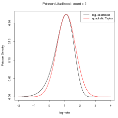
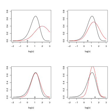
An important point to note here is that the log-likelihood is a function of the parameters X given the data Y . This is what is approximated with a quadratic in X. Likelihoods that are not approximately quadratic as functions of the data given the parameters (such as common probability mass functions like the Poisson, the Binomial, etc) are often adequately approximated as quadratic in X. See Figure 4.1.
The posterior mean μ is found by Newton-Raphson or a similar iterative search algorithm. The c terms in Equation (4.6) are simply the second order coefficients of the Taylor series expansion. An important caveat is that the data are modelled as conditionally independent given the parameters; each Taylor series expansion is univariate and thus a simple and fast calculation. Writing the log-likelihood as f�x�, the Taylor series to second order is:
with b � f��x0��f�� �x0�x and c ��f�� �x0� (a is not required). Thus b � f��x0��cx.
The search algorithm for finding the mean μ represents the bulk of the work in finding the Gaussian approximation. Equivalent to Newton-Raphson is iteratively solving the system of linear equations
 | (4.8) |
for μ.
The key to solving this equation fast is that the Markovian structure of QX (and thus
QX �diagc�) leads to the matrix being very sparse. A Cholesky decomposition of a
matrix Q renders the matrix as the product of a lower triangular matrix with its own
transpose:
 | (4.9) |
Solving Equation (4.8) for μ then amounts to solving Lv � b for v and then solving LT μ � v for μ. All calculations are swift and potentially large matrices may be stored cheaply due to sparseness and lower diagonality.
The Taylor series expansion is most accurate if centred on the mode (mean) of the posterior. Therefore, at each iteration of the search algorithm, the Taylor series is recalculated. This still represents a small number of computational steps as the algorithm typically converges quickly (less than 10 iterations for even very large problems, such as 104 parameters with precision matrices of order 104 � 104).
A simple toy example illustrates the Gaussian approximation. For a single Poisson count y � 3 the objective is to construct the posterior probability distribution for the rate. As the rate is strictly positive, a log-link is used and the log-rate x is inferred.
A diffuse Gaussian prior on x with mean zero and precision κ of 0.001 (variance � 1sκ of 103) is placed on the log-rate parameter. The likelihood is assumed to be Poisson. As the problem is univariate, numerical integration is easily used to determine the posterior for the log-rate. Gaussian approximations formed by expanding a second order Taylor series around 4 different values of the log-rate are shown for comparison in Figure 4.2.
The posterior distribution is then
To approximate this we construct a quadratic Taylor expansion of the unnormalised
log-likelihood yx � expx� around a suitable x0. The univariate approximation is
now
 | (4.11) |
which is in the form of a Normal distribution with mean  and variance
and from Equation (4.7):
The mode x0 is found by iterating the Taylor series expansion with setting
x0 �c � κ�b. This is equivalent to using Newton-Raphson to find the mode of the
posterior. Convergence for this example takes only two steps.
|
|
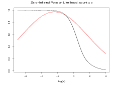
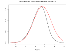
Even if the quadratic approximation to the log-likelihood is poor, the posterior approximation may be good. An example of this is when the likelihood is a zero-inflated Poisson (see Section 2.4 and Equation (2.18)) given by
 | (4.13) |
with q � logit�1x� and λ � ex.
Although the likelihood as a function of count y is bimodal (a mixture of a point mass at zero and a Poisson), as a function of the log-rate x it is unimodal. However, it is very skewed and thus the quadratic approximation to the likelihood is poor; see Figure 4.3(a). The posterior, even under a diffuse prior, is necessarily much less skewed and thus the Gaussian approximation to the posterior is much better; Figure 4.3(b).
|
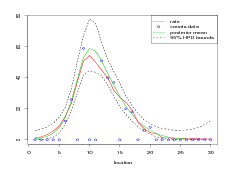
A multivariate example shows the difference between inference using a GMRF approximation and MCMC sampling. A smooth (Gaussian) curve X is defined at regular points in a 1-dimensional space. Counts data are generated from a zero-inflated Poisson with rate parameter given by the exponential of the smooth curve and probability of potential presence given by the inverse logit:
 | (4.14) |
with qj � and λj � exj.
An intrinsic GMRF prior is placed on X with precision matrix given by
 | (4.15) |
where R is as per Equation 2.11 and κ is set to ensure smoothness of the curve across the locations.
The goal is then to infer the posterior πXSY �:
Both a Metropolis Hastings MCMC algorithm and a GMRF approximation were coded and the results for both appear in Figure 4.4. There are 30 locations, regularly spaced, with counts data generated for each of them. To run an MCMC chain of length 3 � 105 for the 30 latent parameters took about 4 minutes. In contrast, it took just under a fifth of a second to fit the GMRF approximation. This represents a speedup in performance of around 3 orders of magnitude for similar results. Even then, the MCMC sampler was started in the correct place to avoid burn in and the code was optimised and tweaked to achieve a good acceptance rate for the proposals.
|
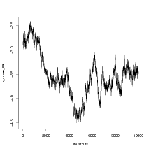
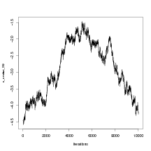
The most obvious difference between the two Figures is to the right hand side. It appears that the GMRF approximation is overestimating the response (which is very low) in this region. However, examination of the trace plot for the log of the response shows that in fact, the Metropolis-Hastings routine is mixing poorly in that region (Figure 4.5). This is an illustration of why it is not correct to assume an MCMC sampler is doing a better job of approximating the posterior than the GMRF approximation.
|
|
Section 4.1.1 shows how the Gaussian approximation may be applied even to models with mixture likelihoods, such as a zero-modified distribution. A multivariate example of this is shown in Section 4.1.1, where a GMRF prior and zero-inflated Poisson likelihood yield a posterior that is adequately approximated by a GMRF. In this example, the rate and the probability of potential presence are both functions of a single stochastic process.
It will be shown in Chapter 6 that such a model is suitable in the context of pollen based ecology. Where such a model is unsuitable, two separate processes should be modelled; one for the response and another for the probability of presence. However, such a model is unsuited to approximation with a GMRF. That each datum depends only on a single parameter is a central assumption (or modelling choice) in fitting such approximations. This is because approximating the likelihood with a quadratic requires the function to be univariate in the latent parameter; a second order Taylor series expansion for a bivariate function has 8 terms, compared to 2 for an expansion of a univariate function.
In some cases, such as the incorporation of zero-mean random effects, the model may simply be reparameterised so that each datum depends on a single parameter, which is the sum of the spatial part plus the non-spatial random effect (see Rue and Held (2005), Chapter 1). This typically leads to a graph / GMRF of double the size and thus double the number of parameters, but is not a fundamental obstacle to the implementation of the approximation.
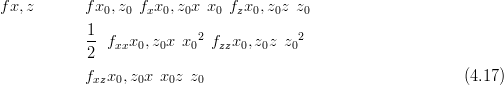
However, a similar reparameterisation does not exist for the zero-modified distribution; the likelihood necessarily depends on two distinct parameters. To see this, if the zero-inflated counts data depend on, say, x for the response when present and z for the probability of potential presence, then the second order Taylor series expansion of the log-likelihood f�x,z� is
where fx is the first order derivative w.r.t. x of f, fz is the first order derivative w.r.t. z of f, fxx is the second order derivative w.r.t. x of f, fzz is the second order derivative w.r.t. z of f and fxz is .
.
This cannot be re-expressed as a function of a single variable. The Taylor series
remains multidimensional and is cumbersome. Equation (4.17) cannot be expressed as
y � y0�T QY y � y0� and is therefore incompatible with the GMRF approximation
technique.
In the case of a single underlying process controlling both response and the probability of potential presence, modelling two separate spatial processes will necessarily perform worse than modelling the single process. For example, if MCMC methods are used, the two spatial parts will be very highly correlated (as they in fact arise from a single process), leading to poor mixing, as shown in Figure 4.6. This is a consequence of the overparameterisation of the model.
|
|
A note on zero-inflated models lying on a grid: The GMRF approximation method requires all calculations to be defined on a grid across the locations space (due to the Markov structure). In Rue and Held (2005) and Rue et al. (2008), the authors advocate pushing each datapoint to the nearest gridpoint. This will typically keep the locations within the measurement error as the granularity of the grid may be very large. When two or more datapoints are closest to the same grid-point they are simply aggregated or averaged. However, this has implications for zero-inflated counts data as the distributions are not closed under addition. Therefore, in this thesis, the data are pushed to the nearest gridpoint but are kept separate so that there may be multiple counts per gridpoint.
In a hierarchical model, some of the hyperparameters may be unknown. They must be
treated as random variables and inferred from the data. An MCMC algorithm will
typically sample from the joint posterior for the parameters and the hyperparameters
given the data πX,θSY �. This posterior may also be expressed as the product of the
marginal posterior for the hyperparameters πθSY � and the posterior for the parameters
given the hyperparameters πXSθ,Y �:
 | (4.18) |
The objective then is to find πθSY � and πXSθ,Y �. Re-expressing Equation (4.18)
as
 | (4.19) |
and using a GMRF approximation for the denominator πXSθ,Y � gives the Laplace
approximation
for the posterior of the hyperparameters:
 | (4.20) |
and writing the numerator in closed form, up to proportionality constant gives
 | (4.21) |
where πLθSY � is called the Laplace approximation to the posterior.
As stated previously, the type of problem to which the INLA routine is well suited is
one in which the hyperparameters are essentially nuisance parameters. It is
acceptable to treat them crudely, with a view to integrating them out entirely.
Evaluating Equation (4.21) at a number of discrete points on a grid over all θ is the
approach taken in Rue et al. (2008). The normalised approximate posterior πLθSY �
is found by summing Equation (4.21) across the points and dividing by the
sum.
The marginal posterior for the parameters is then simply the weighted sum over all the discrete points in θ space:
 | (4.22) |
where δk are area weights, depending on the not-necessarily uniform discrete spacings in the θ space. This is only possible for low dimensional θ, otherwise the numerical integration quickly becomes difficult as the number of gridpoint grows as ND, where N is the number of points along a particular component of θ and D is the number of components of θ.
Rue et al. (2008) shows that this is a good approximation for a wide range of statistical problem. It is sufficient to note that the MCMC alternative is cumbersome to the point of rendering it impractical. The hyperparameters are often highly correlated with the parameters; e.g. the smoothness hyperparameter and associated latent field random variables. Thus a Metropolis-Hastings algorithm will suffer from serious mixing problems unless a tailored block-update proposal mechanism is built.
A further approximation is to use the modal value of the hyperparameters. The hyperparameters are then considered known, having been inferred from the data for the purpose of constructing the marginal posterior for the parameters given the data (maximum a-posteriori selection of hyperparameters; see, for example Oakley and O’Hagan (2002)).
This approximation is motivated by the inverse problem application central to this thesis. In order to invert the model and construct inverse predictive distributions for unknown hyperparameters, the model must be inverted (inverse problem) for each value on the discrete grid of hyperparameters. The marginal distribution for the posterior of the parameters given the data only is represented as a mixture of Gaussians (Equation (4.22)). This is itself modelled non-parametrically and a numerical integration step would be added to each marginal likelihood calculation for the inverse predictive procedure.
The decision on whether to integrate out the hyperparameters or to simply use the modal values of the hyperparameters is a trade off between speed and accuracy. The decision is context specific, depending not only on the data and the model used and the number of hyperparameters, but also the task that is being performed. For example, in order to perform actual inverse predictions given counts data the gain in accuracy associated with integrating over the hyperparameters may well justify the additional effort, which is not great.
In cross-validation terms, however, the increase in computation is enormous, as there will be k replications where k is the number of datapoints; furthermore, the modal approximation will place the bulk of the probability mass in the correct location so that the inverse predictive distributions are approximately equal for parameters given fixed (modal) hyperparameters and the marginal parameters. Therefore, use of hyperparameters fixed at their modal posterior values is advocated for the task of cross-validation. This is discussed for the pollen dataset in Section 6.4.1, with results.
If the posterior for an individual latent parameter (individual location on the
non-parametric latent field) given the hyperparameters  xjSθk,Y � is required, then the
simplest univariate approximation is the marginal Gaussian, taken from the joint GMRF
approximation. This is already constructed when finding the Laplace approximation for
the hyperparameters posterior and is therefore very cheap. The marginal variances are
computed using a fast recursion algorithm applied to the already available Cholesky
decomposition of the joint precision matrix (see Rue and Held (2005) or Rue
et al. (2008)).
xjSθk,Y � is required, then the
simplest univariate approximation is the marginal Gaussian, taken from the joint GMRF
approximation. This is already constructed when finding the Laplace approximation for
the hyperparameters posterior and is therefore very cheap. The marginal variances are
computed using a fast recursion algorithm applied to the already available Cholesky
decomposition of the joint precision matrix (see Rue and Held (2005) or Rue
et al. (2008)).
When more accurate approximations are required, there is a Laplace approximation for the marginal distributions of the parameters given by (Rue et al. (2008))
 | (4.23) |
where  GGX�jSxj,Y,θk� is a Gaussian approximation to the conditional posterior for
all X except xj, evaluated at the kth point of the discrete grid over θ. This Laplace
approximation involves re-fitting a GMRF approximation for each θk and each xj and is
thus expensive computationally.
GGX�jSxj,Y,θk� is a Gaussian approximation to the conditional posterior for
all X except xj, evaluated at the kth point of the discrete grid over θ. This Laplace
approximation involves re-fitting a GMRF approximation for each θk and each xj and is
thus expensive computationally.
Approximations to this approximation may be made, such as fitting a skew-normal via a third order Taylor expansion (called a Simplified Laplace Approximation in Rue et al. (2008)). Both the computational effort and the accuracy will fall between the Gaussian approximation and the full Laplace approximation. This leads to a method of checking the accuracy of the approximations: If the Kullback-Leibler divergence between Equation (4.22) using the Gaussian and the Simplified Laplace approximations is small, then both are deemed acceptable. Otherwise, the Kullback-Leibler divergence between the Simplified Laplace and Laplace approximation versions of Equation (4.22) are similarly compared. If these again differ, then the Laplace is the best estimate, but adequacy of the approximation is not determined (see again Rue et al. (2008)).
Of course, if the one of these more accurate approximations are calculated in order to assess the relative accuracy of the Gaussian approximation then they should simply be used instead. The computational convenience of the simpler Gaussian approximation is then lost. An intermediary solution is to calculate the more accurate approximations at a random subset of points; the accuracy of the Gaussian approximation at these locations then gives an indication of the accuracy across all locations. If the Gaussian approximation is thereby deemed to be of insufficient accuracy then the more accurate approximations are required.
The method of checking the accuracy of the approximations given above is for the forward problem. The interest here is in the inverse problem; if the Gaussian approximation and the more accurate (but more costly) Laplace type approximations give the same answer for the inverse predictive distributions, then there is no gain. This is an indication that the Gaussian approximation is sufficiently accurate for the requirements of the inverse problem.
In order to invert the model, the marginal posteriors must be calculated at all locations. In regions of little data, the GMRF prior will dominate and the posterior will be close to GMRF (in regions of no data, the posterior will converge to the prior). Where there is an abundance of data, the Central Limit Theorem will apply and, again, the posterior will be approximately Gaussian. The Simplified Laplace involves a third order term for the Taylor series approximation to the posterior; this is the skew term. Only if the marginal posterior in a given location has significant skew will the Laplace approximation be closer to the actual posterior than the Gaussian approximation.
Model comparison and evaluation is of fundamental concern in all statistical data analysis. As previously stated, the concern here is in the inverse problem (predicting input variable from a given model output variable). For this reason, model evaluation in the inverse sense is the main focus. Specifically, the ability of the model to successfully reconstruct or predict the correct location of a new count (or vector of counts) is what determines the usefulness of the model.
As a never ending supply of new data is not available and the model will ultimately be
used to make unverifiable reconstructions, validation must be done on the same training
data set to which the forward model is fitted. Cross-validation is a common technique for
assessing the model fit to data. M-fold cross-validation refers to the practice of leaving
out a subset of the data (1sM of all the training dataset); the model is fitted to the
remaining data (M � 1�sM of the total) and the ability of the model to predict (or
reconstruct) the remaining data is assessed. The concern here is with leave-one-out cross
validation; this involves refitting the model to all but one datum and then assessing the
ability of the model to predict the single left out point. This must be repeated
M times, where M is the total number of datapoints (7742 in the motivating
palaeoclimate problem). From here on, leave-one-out cross-validation will simply be
referred to as cross-validation as this will be the only form of cross-validation
considered.
Performing cross-validation in the forward sense for the palaeoclimate problem involves fitting the model to all but a single pollen count (or assemblage) and then predicting that count (or assemblage), given the associated climate (location in climate space). Cross-validation in the inverse sense is more appropriate. The main reason for this is that the ultimate goal of the project is to make inferences on climate, given a vector of fossil pollen counts.
Interest here therefore lies in forming the leave-one-out inverse cross-validation predictive posteriors for the locations. These are then compared in some way with the actual observed values. So, for each observation j:
In either case, the main difficulty in performing cross-validation is computational. For example, to perform exact cross-validation using a brute-force approach involves fitting the model M times, where M is the number of datapoints. The motivating palaeoclimate problem has just under eight thousand modern / training data collection sites. Given that an MCMC sample of the saturated posterior (the posterior of the parameters given all training data data) takes of the order of two weeks to run, eight thousand replications would take 300 years. Some existing techniques are introduced in Section 4.2.1. A new approach for the cross-validation in the inverse sense, made possible by the closed form of the forward model posteriors, is explored in Section 4.2.3. This represents a novel contribution to the INLA methodology.
Looking at Equation (4.24), the brute force approach is to compute the leave-one-out
posterior for the responses πXSỸ�j, �j� for each left-out datum pair �lj,yj�. The
integral on the right hand side of Equation (4.24) must then be computed for
each j and this represents further computational labour as it is an intractable
integral. The contribution in this work is to deliver a method for fast updates
to the saturated posterior (available in closed form via the INLA method) to
be made. The leave-one-out posteriors are thus available without needing to
recompute the INLA approximations for each leave-one-out subset of the data.
This novel extension of the INLA methodology is detailed in Section 4.2.3 and
is a consequence of the Multivariate-Normal form of the GMRF posterior for
X.
�j� for each left-out datum pair �lj,yj�. The
integral on the right hand side of Equation (4.24) must then be computed for
each j and this represents further computational labour as it is an intractable
integral. The contribution in this work is to deliver a method for fast updates
to the saturated posterior (available in closed form via the INLA method) to
be made. The leave-one-out posteriors are thus available without needing to
recompute the INLA approximations for each leave-one-out subset of the data.
This novel extension of the INLA methodology is detailed in Section 4.2.3 and
is a consequence of the Multivariate-Normal form of the GMRF posterior for
X.
The other challenge in performing cross-validation is how to summarise the model fit. There are many alternatives, some of which are described in Section 4.2.5.
There is a large literature on performing fast Bayesian cross-validations for the forward problem that focus on methods for speeding up the MCMC re-runs. One approach involves using importance resampling. (see, for example, a review in Bhattacharya and Haslett (2008)).
Using an idea that first appeared in Gelfand et al. (1992), samples from the saturated
posterior are re-used so that MCMC is not needed for the leave-one-out cross-validations.
Specifically, if the data are �Y,L� (outputs and inputs to the model, respectively) and the
Bayesian hierarchical model is fitted via MCMC sampling of the latent parameters X,
then the saturated posterior is πXSY,L�. This gives the importance sampling
distribution.
For a particular left out datum yj, the posterior predictive distribution πySlj,L�j,Y �j� is
desired. This is calculated from the integral
 | (4.25) |
Integration is via MCMC. Following the notation in Vehtari and Lampinen (2002), if
samples from πXSL�j,Y �j� are available - denoted Ẋh - then a sample ẏh from
πySlj,Ẋjh� is a sample from πySlj,L�j,Y �j�. But πXSL�j,Y �j� is the undesirable
MCMC repetition. A sample from this distribution is more easily obtained through
importance resampling; if Xh is a sample from the saturated posterior πXSL,Y �, then
samples Ẋh may be obtained by resampling Ẋh with importance weights given
by
 | (4.26) |
This is analytically available, since it is the likelihood function with known parameters. The weights are thus simple and quick to calculate and samples from the importance sampling distribution (the saturated posterior) are already available from the initial MCMC run.
When model inputs L are of lower dimension than outputs Y , cross-validation of the inverse problem may offer an appealing alternative to forward cross-validation. Discrepancy measures between the data and the corresponding predictive densities are computed; these measures are easier to construct and interpret for the lower dimensional variable. Furthermore, when the ultimate interest is in predicting l for a given y (the inverse problem), then inverse cross-validation is more appropriate.
However, there is very little literature on cross-validation in inverse problems. In fact, according to Bhattacharya (2004)
“we do not know of any paper that discusses cross-validation in the context of inverse problems”
Therefore, the technique introduced in Bhattacharya (2004) and presented in detail in Bhattacharya and Haslett (2008), provides the only benchmark. In that paper, the authors point out that importance weights for the inverse problem are not tractable calculations. They suggest using a posterior for a single left-out point (obtained via regular MCMC) as the importance sampling density and show how to calculate the importance weights for the other points. Sampling without replacement is also advocated, to protect against highly variable importance weights. They call the algorithm Importance Re-sampling MCMC or IRMCMC.
Although there is still an MCMC step in the IRMCMC algorithm, it is of much lower dimension than re-running MCMC for each left out point. Another important detail is the choice of the initial left-out point; Bhattacharya and Haslett (2008) demonstrate methods for making this choice.
For cross-validation in inverse problems, IRMCMC not only runs much faster than doing multiple regular MCMC runs, but it also achieves superior mixing (and thus more accurate results). This is due to the low dimensionality of the inverse problem, compared to the forward problem. The MCMC runs in the IRMCMC algorithm explore the typically multimodal target distribution of l better as updates for X do not have to be run in parallel (see Bhattacharya and Haslett (2008) for discussion and examples). In fact, IRMCMC may be thought of as regular MCMC with a special proposal mechanism.
The INLA method introduced in Section 4.1 delivers closed-form approximations to
the saturated posterior for the latent parameters X. The same weightings in
Equation (4.26) may again be used to perform forward cross-validation without MCMC.
The marginal saturated posterior πxjSL,Y � (available analytically) is weighted
using Equation (4.26) and the uni-dimensional integral in Equation (4.25 is
computed using fast numerical methods, such as Gauss-Hermite quadrature (see Rue
et al. (2008)).
This section introduces a novel method for fast inverse cross-validation using the INLA methods. When the saturated posterior for the latent parameters X is approximated with a GMRF (as per Section 4.1.1) then augmenting this posterior to correct for a left-out datum is straightforward. The posterior is entirely specified by the first two moments; fast updates to these to correct for left out data negates the need to re-fit the entire model.
If both the prior and the posterior are multivariate normal, then the posterior covariance matrix is given by
 | (4.27) |
where Q is the prior precision matrix and R is the likelihood precision matrix and is diagonal.
The posterior covariance matrix for the case of leaving out the jth point is similarly given by
 | (4.28) |
where rj is the precision of the jth datum and Ij is a square matrix of zeros with a one at the jjth entry.
If for some scalar γj,
 | (4.29) |
then the covariance matrix for all data except any left-out point j may be found without additional inversion of the precision matrix.
γj is found by post multiplying both sides of Equation (4.29) by Σ�j�1 as per Equation (4.28) gives
which only holds if
 | (4.31) |
The posterior mean is found via
 | (4.32) |
which becomes
Hence, for multivariate normal prior and likelihood, the augmented posterior moments are calculated using fast matrix-vector products with a few scalar calculations. In fact, inversion of the precision matrix may be avoided altogether; only the marginal means and variances are required in cross-validation. The marginal variances are quickly calculated from the Cholesky decomposition of the (sparse) precision matrix Q � R. The updated mean is found by solving the equation
 | (4.34) |
for ν. Given the Cholesky decomposition of Q � R�� LLT , the solution is by
forward-solving and then back-solving two sparse systems of linear equations (as per the
solution of Equation (4.8) and is thus very fast. Now the updated mean is given
by
 | (4.35) |
The marginal variances are the diagonal of the covariance matrix and are found via
where the required elements of Σ are found directly from the Cholesky decomposition of the precision matrix Q�R and �Σj,,Σ,j� denotes the jth row and column of Σ respectively. 1
In the more general case of non-Gaussian likelihoods for counts data, the posterior is approximated as a GMRF and the same shortcuts may be applied, with appropriate changes. Augmenting the posterior distribution of the latent parameters to correct for leaving out a single datum is again both fast and exact (given the saturated posterior approximation with a GMRF). Due to the transform generally required between the latent unconstrained parameters and the expectation of the counts data, the above equations require adaptation.
Recall that in the context of the GMRF approximation the posterior mean for the latent parameters is given by
 | (4.37) |
where b is the first order coefficient in the Taylor series expansion of the
log-likelihood and c is the second order coefficient. Solving this equation for μ is fast due
to the sparse structure of the posterior precision matrix Q � diagc�, which is
decomposed as LLT . Correcting the vectors b and c to leave out a single datum at
position j is extremely fast as only the jth element is changed. If there is only a
single count at j, then both bj and cj are exactly zero. Otherwise, the Taylor
expansion of the log-likelihood of the remaining counts at j is calculated to
get b�j and c�j at j; but this is a univariate problem and thus very simple and
fast.
The augmented mean is then a case of solving
 | (4.38) |
for μ�j (note that the prior precision matrix Q is unchanged).
Furthermore, the multidimensional optimization step required to find the mode around which the Taylor expansions are computed may be entirely avoided. The Taylor series will be accurate provided the expansion is centred approximately around the mode. The saturated posterior provides a good approximation and is already available. Thus extra expensive, iterative searches for the mode (optimization) are not required.
Cross-validation of the forward problem is markedly different from the inverse problem. In the forward problem, the leave-one-out predictive distribution of a count given location is required; therefore only the marginal posterior of the latent parameter at that known location requires augmentation to account for the left out point. This is thus a univariate problem.
Furthermore, as the likelihood normalising constant is known, the ratio of the leave-one-out posterior to the saturated posterior is given by the (inverse of the) marginal likelihood, which is a known function. This fact is exploited in sampling based cross-validation for the quick calculation of importance sampling weights (see Section 4.2.1).
Rue et al. (2008) also use this ratio for cross-validation of the forward problem in the context of the INLA method. The marginal posterior for the parameter X at location i when datum yi is removed is quickly and easily found as
 | (4.39) |
where πxiSY � is the marginal saturated posterior.
As this is univariate, integration and thus normalisation are available numerically.
The inverse problem is more difficult; dropping a datapoint now requires the construction of the predictive distribution across all locations, given the left out count and the updated posterior. The normalising constant must be found by calculating this across all possible locations, so that even if the cross-validation summary statistic is a function of the value of the predictive distribution at the correct location alone, it must still be calculated everywhere.
Inverse cross-validation is more closely related to the fast rank-one updates described in Rue et al. (2008) to compute the posterior multivariate normal mean, conditioned on a fixed value of the parameter at a single point. These fast updates are used for the computation of the Laplace approximation for the marginals of the model parameters (see Section 4.1.4). This task is, at first glance, very different from the task of inverse cross-validation; however, some of the same methodology is applied.
Both tasks could be completed through a re-fitting of the entire model but in both cases this computationally intensive option may be avoided by instead correcting (updating) the moments of the saturated posterior. As in that paper, a multidimensional optimization step is avoided; the saturated posterior mean (mode) is used as an approximation to the updated mode. As shown above, the Taylor series coefficients b and c are recalculated quickly as they are only required for a single point; centering the expansion around the approximated mode avoids the multidimensional optimization.
It should be noted here that these fast updates to the posterior moments assume that the joint posterior, across all locations, is available; this is only the case for the GMRF approximation to the latent parameters. If the Laplace approximation is used for all the latent parameters, this gives disjoint, albeit potentially more accurate, approximations for the posterior marginals only. This approximation is not amenable to fast updating of the saturated posterior for leave-one-out cross-validation as updates must be performed on a closed-form joint posterior for X.
The calculations in Equations (4.29) and (4.40) may be sped up by observing that the effect of removing a datapoint is local. Rue et al. (2008) calls the area effected by changes to a point / location the “region of interest”. The moments need only be changed within this region of interest, so that correcting the saturated posterior involves only a few, fast calculations. The region of interest may be found by working out from the location of the left-out point until changes to the moments drop below a certain threshold or by using preset distances to specify the region. Depending on the size of the preset and fixed region, the latter involves fewer calculations and is thus faster, but may represent an approximate cross-validation if the region is set too small.
Solving Equation (4.38) using the same method as per finding the saturated posterior requires a fresh Cholesky decomposition of the posterior precision matrix; unfortunately L�j is not calculable directly from L. In addition, the marginal variances given by Equation (4.36) require computation of an entire row (or column; the matrix is symmetric) of the joint covariance matrix. Repeating for each left out point therefore ultimately involves computing the entire saturated posterior covariance matrix.
If the entire saturated posterior covariance matrix is calculated then updates to this matrix are given using Equation (4.29). This is the preferred approach as the computations associated with a once off full inversion are less than that associated with solving Equation (4.38) and finding, via recursion, the marginal variances. The posterior mean, corrected for a left-out point is then given directly by a simple matrix-vector product:
 | (4.40) |
In the context of the GMRF approximation the γj required in Equation (4.29) is given by
 | (4.41) |
Leaving out data at a single point will have minimal effect on the posterior for the hyperparameters. Therefore, the approximation that there is no effect on the hyperparameters is adopted here. The accuracy of this approximation may be tested by leaving out a datapoint and refitting the Laplace approximation for the posterior of the hyperparameters. Comparison with the saturated hyperparameter posterior will show no (negligible) difference if this approximation is accurate. In the limit of infinite (large amounts of) data, this approximation is exact.
Given the above methods for augmenting the posterior moments of the latent parameters, the main computational burden in performing inverse cross-validation is in constructing the inverse posterior predictive distributions. As these are often multimodal in shape (see Section 2.5.1), they cannot be well approximated with a deterministic distribution. MCMC is the most obvious choice, as per Haslett et al. (2006) and Bhattacharya and Haslett (2008); however a faster alternative is presented here.
The approximation to the posterior of the latent parameters requires the imposition of a discrete grid on the locations space. The inverse predictive distributions are therefore discrete. Hence, Monte-Carlo may again be avoided; the un-normalised posterior predictive distribution for the locations are calculated at all points on the grid. Dividing by the sum normalizes the mass function.
The multimodal nature of these distributions is a fundamental challenge to any MCMC sampling algorithm (see for example Bhattacharya and Haslett (2008)) as the Markov chain may become stuck in one mode and fail to explore others. The fine grid necessitated by the GMRF approximation fortunately eliminates this problem.
Having performed inverse cross-validation, a summary statistic is required to report the “fit” of the model to the data. Bhattacharya (2004) advocates using reference distributions. A discrepancy measure is computed between samples drawn from the cross-validation leave-one-out posteriors and the corresponding observations. Four such discrepancy measures are presented in that work; the first three are measures of the “distance” between the mode of the posterior predictive distribution and the observed value, standardised by the variance of the predictive distribution. The sum of these values is labeled the observed discrepancy. The reference distribution is then the distribution of the discrepancy measure with the modal values replaced with samples from the posterior predictive distributions. The model is said to fit the data if the observed discrepancy is within the 95% highest density region of the reference distribution. Bhattacharya (2004) also notes, however, that “there seems to exist no easily computable reference distribution” for this statistic.
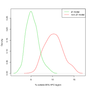
Although the reference distributions themselves are unimodal, the discrepancy measures used in Bhattacharya (2004) are a poor summary of the fit to data of the multimodal predictive distributions. The percentage of observations falling outside the corresponding 95% highest posterior predictive distribution is a useful statistic here. This will be approximately 5% if the model fits the data, regardless of the shape of the predictive distribution.
Definition 5 Δ is the percentage of locations that fall outside the 95% highest posterior density region of their leave-one-out cross-validation inverse posterior predictive distribution.
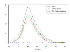
Repeated runs of a toy model illustrate the cross-validation summary statistic given in Definition 5. Counts data are simulated from a known distribution function, defined on a 15 � 15 regular lattice. Leave-one-out cross-validation is performed in the inverse sense and the percentage of points falling outside the 95% highest posterior density region of the predictive distribution is calculated. Cross-validation is performed using the fast updates to the saturated posterior moments derived in Section 4.2.3; however, these fast corrections are exact, given the GMRF approximation. Once the modal values of the hyperparameters are found using the Laplace approximation, they are considered fixed for the cross-validation procedure.
The toy example algorithm is:
The results for this exercise are shown in Figure 4.7 with M � 300.
|
|
This chapter has introduced the application of approximation techniques (INLA) to inverse problems. The approximations apply to the forward problem, negating the need for MCMC type inference and returning closed form posteriors. This represents a speed up of several orders of magnitude in the fitting the forward model to the training data.
Spatial zero-inflated models in which there are two entirely separate latent processes are not compatible with the INLA method. However, a single-process model for zero-inflated counts data in which probability of presence and abundance when present are modelled as functions of a single underlying process is well suited to the technique. In fact, this model was developed before the INLA method was considered as it will lead to faster and more accurate inferences than the two-process model under MCMC, provided the model is correct.
Although model validation is the subject of a very extensive literature for the forward problem, the inverse problem has rarely been considered. MCMC based cross-validation is computationally intensive in the extreme; Bhattacharya and Haslett (2008) sets the standard for this research by augmenting MCMC based validations with importance resampling to greatly speed up calculations. However, this approach still requires much computation; although running times for an example palaeoclimate problem are reduced by several orders of magnitude, the cross-validation still takes hours or even days to run.
This computational burden hampers the comparison of multiple models. A method for performing inverse cross-validation is therefore introduced. This method fits the saturated posterior for the forward model using the INLA method. The hierarchical hyperparameters are fixed at their posterior modal values and a new, very fast method for correcting the posterior for the parameters is applied. This allows for fast calculations of the leave-one-out posterior for the forward problem. The inverse predictive distributions are also found without resorting to sampling methods; this is due to the imposition of a discrete grid in the forward fitting stage.
Observing that corrections to the saturated posterior are only necessary in a local region speeds up the cross-validation further. For the motivating palaeoclimate problem, inverse cross-validation now takes around one hour using these methods. The estimated running time using brute-force MCMC re-runs is of the order of many years; even the fast importance sampling method that set the current standard takes about two weeks (although most of that is taken in running the initial regular MCMC chain). These vast improvements in speed are coupled with improvements in the method also; hyperparameters are no longer fixed a-priori but are estimated from the data.
The advancements in the modelling of the pollen data since Haslett et al. (2006) are therefore as follows: