In order to set the context of the work in this thesis, a brief palaeoclimate reconstruction literature review is conducted in Section 2.1. Gaps in the existing methodology are identified and solutions developed in this thesis are introduced.
The contributions are relevant to a wider statistical methodology beyond palaeoclimate reconstruction; Section 2.2 discusses Bayesian methods that are relevant to the methodology developed in this thesis. Section 2.4 introduces explicit modelling of zero-inflated counts data. Section 2.5 defines inverse regression and demonstrates the generic challenge of such problems with a simple example. Section 2.6 begins the discussion of how models of this type are evaluated and compared, focusing on inverse problems.
Although the contributions made in this thesis to both statistical modelling and inference are applicable to a variety of problems, it is most natural to set them in the context of the motivating problem of statistical palaeoclimate reconstruction using pollen data.
Throughout the later chapters, existing methodology is referenced as required. Therefore, a brief and focussed review of the palaeoclimate literature only is conducted here in order to motivate and frame the work in this thesis.
Detailed reviews are already available; see ter Braak (1995) for a review of non-Bayesian palaeoecology, Haslett et al. (2006) for a review of Bayesian and non-Bayesian palaeoclimate reconstruction and Bhattacharya (2004) for details on Bayesian inference in inverse problems with a focus on palaeoclimate reconstruction. It is not a worthwhile exercise to reproduce these in detail here; an overview, drawing directly from these and other sources is sufficient. Details may be found in the references.
The outline for the literature review is as follows:
Unfortunately, the terminology used in palaeoclimate statistics has become somewhat confused. ter Braak (1995) categorises non-Bayesian approaches into two distinct paradigms, which he terms “classical” and “inverse”. The former refers to regression of ecological data on climate. The latter is vice-versa; hence the label inverse as cause and effect have been inverted. “Classical” reconstruction may be thought of as building a forward (cause implies effect) model and subsequently inverting the model to find cause given effect. This use of “inverse” reconstruction involves the simpler task of regression of cause (climate) on effect (ecology).
Haslett et al. (2006) and Bhattacharya (2004) do not consider the ter Braak (1995) definition of “inverse” modelling and use the term “classical” to refer to all non-Bayesian approaches. “Inverse” modelling in these works refers to the inversion of a forward model, Bayesian or otherwise. “Forward” models are equivalent to the models calibrated on the modern data in the “classical” approach of ter Braak (1995).
This is the terminology adopted here; thus quotation marks for these definitions of “forward”, “inverse” and “classical” will be dropped from here on; the ter Braak (1995) definition of “inverse” will be referred to as classical inverse.
ter Braak (1995) notes that palaeoclimate reconstruction is a highly non-linear multivariate calibration problem. Although climate reconstruction from modern and fossil pollen is taken as the only worked example, the author notes that the techniques carry over immediately to calibration in other areas of palaeoecology.
He uses the interesting phrase
“the present day calibration is used to infer the past climate”
to broadly describe the way that all statistical climate reconstruction techniques work. The contribution of this thesis mainly lies in the calibration of such data (spatial, compositional, zero-inflated counts). The focus is in building and assessing the models.
It is worth noting that although Krutchkoff (1967) claims the superiority of this definition of the classical inverse method in predictive power, ter Braak (1995) shows that this approach is only slightly better when samples are from a large central part of the distribution of the training set. The inversion of the forward model is considerably better at the extremes. The classical inverse method also treats each climate variable separately and independently; a surprising and illogical model. In the Bayesian context, it is more natural to build forward (cause implies effect) models and invert using Bayes rule.
The classical palaeoclimate modelling approach may be split into three approaches:
The second two are classical inverse methods and are not considered further (the third method is a direct calibration of climate on pollen). The response surface method is the closest in spirit to the approach introduced in the Bayesian sense by Haslett et al. (2006) and developed here. Response surface methods typically use least squares based methods to regress pollen on climate; this relationship is then inverted to produce inference on fossil climate given pollen. Bartlein et al. (1986) used cubic polynomials in two climate dimensions fitted to observed percentages of eight pollen types. The authors encountered two difficulties with their approach:
Both of these problems were addressed through switching from fitting cubic polynomial response functions to non-parametric responses. Prentice et al. (1991) used local weighted averaging to fit smooth non-parametric surfaces to the data. This technique has since been followed by Huntley (1993) and others and is the closest non-Bayesian equivalent to the model of Haslett et al. (2006).
This method posed the question of what to do with the problem of multiple modern analogues. In fact, this problem is common for inverse problems (see Section 2.5.1). In the method of Allen et al. (2000), the locations in climate space of the ten “nearest” response surface to the compositional fossil vector were averaged. This was an attempt to provide a single location as the most likely reconstructed climate. However, it can be a most unsatisfactory approach; in the simplest example, a plant type that is abundant in the centre of climate space will send the signal “not close to centre” when the fossil record has low pollen counts of this type. The ten nearest response surface values will come from the edges of climate space. Averaging these ten locations in climate space will then reconstruct the centre; i.e. the very place that the signal most strongly rejects!
A Bayesian approach offers a solution to the above problems. Uncertainty is handled in a consistent manner and full posterior distributions on random variables of interest may be summarised in any way desired. So, for the above example, the posterior distribution would be multimodal with lowest probability assigned to the area in which the pollen type is scarce; an honest assessment of belief in light of the low signal.
The Bayesian paradigm (Section 2.2) has been applied to palaeoclimate reconstruction; however, the literature is “very small and scattered” (Haslett et al. (2006)). The first detailed Bayesian methodology comes from a series of papers by a group in the University of Helsinki (Vasko et al. (2000), Toivonen et al. (2001) and Korhola et al. (2002)). However, they work with a single climate variable and use a unimodal response with a functional form, invoking Shelford’s law of tolerance , which states that a species thrives best at a particular value of an environmental variable (optimum) and cannot survive if this variable is too high or too low.
Such a response model is inappropriate for many applications of ecology model. For example, Huntley (1993) shows that, for pollen data, multimodal responses in several climate dimensions are common. This is a result of species indistinguishably; most pollen spore types represent several species or even an entire genus.
More recent Bayesian work by Holden et al. (2008) also invoke Shelford’s law. This allows them to avoid MCMC based inference. In that paper, zero-inflation of the data is explicitly modelled; presence and abundance when presence are modelled as functions of a single underlying spatial process. This model is related to the model of Salter-Townshend and Haslett (2006).
Recognizing the issue with multimodal responses, Haslett et al. (2006) applied the non-parametric response surfaces approach of Huntley (1993) in a Bayesian context. A 50 � 50 regular grid was employed across a two dimensional climate space on which modern pollen data were placed; a Gaussian Markov prior on the non-parametric responses defined on this grid ensured the smoothness of the latent responses. This created a model flexible enough to deal with any type of smooth response function.
Although only a subset of the data was examined (14 taxonomic groups were selected by expert opinion from the total set of 48 taxa), the non-parametric approach led to around ten thousand latent random variables. As the posterior for these parameters is only available up to a normalising constant, sampling algorithms (Section 2.2.2) were employed to sample from the posterior. Empirical summary statistics were then used in lieu of theoretical ones.
Computation was found to be the main challenge of the methodology; this in turn led to restrictions on both the complexity of the model and, more importantly, in the validation procedures used to test and compare models. Due to these shortcomings, the paper was presented as a “rather detailed proof of concept” Haslett et al. (2006). A section on issues deferred details some of the shortcomings and the printed discussion with the paper addresses several others.
The work contained in this thesis seeks to address some of these difficulties. Alternative inference techniques are employed, novel to the problem of palaeoclimate reconstruction, in place of the computationally overwhelming sampling algorithms used in Haslett et al. (2006). These techniques yield a normalised posterior on all parameters in closed form; see Section 2.3 for an introduction and Section 4.1 for full details. Assumptions made necessary by computational concerns may be relaxed, leading to a richer model posterior and the availability of more rigorous testing.
The final paragraph of the rejoinder from the authors of Haslett et al. (2006) to the contributed written discussion of the paper ended as follows:
“Zero inflation is a particular challenge …There may well be sampling procedures for the [parameters] that are more efficient than simple random sampling. In short, there remain many methodological challenges.”
In fact, while the authors acknowledge the need to treat the zero counts specially, the model they employ is one for overdispersion only, once again sacrificing model sophistication to computational efficiency.
The avoidance of intensive sampling algorithms allows for more sophisticated models to be developed. In particular, this thesis presents a new model for spatial zero-inflated counts data. The new model is flexible, yet simple. It offers a far more satisfactory account for the extra zeros in the data, yet remains parsimonious.
Model validation did not play a big role in Haslett et al. (2006); leave-one-out cross-validation was presented as a focussed evaluation of the model’s capability to reconstruct climate. A counts vector plus climate space location pair is left out of the modern dataset. The model is trained on the remaining data and the left-out climate is reconstructed using the trained model and the left-out counts vector. This is repeated for each data pairing and summaries of the ability of the model to “predict” the data give a measure of model fit.
However, this would require fitting the model several thousand times. With running times of several weeks, after which the authors concede that “convergence to the correct posterior is far from assured”, repeating the procedure even a dozen times is undesirable to say the least. Therefore, the authors use an approximate cross-validation shortcut; the model, as fit to the entire dataset is used as an approximation to the fit for each left-out point.
In contrast to this, constructing closed form posteriors, using new closed form techniques requires only a few minutes of run time. The development of these techniques is not a contribution in this thesis although application to the area of palaeoclimate reconstruction is novel. Re-fitting the model for each left-out point is now a realistic exercise. Another contribution in this thesis is to quickly correct the entire fitted model to account for leaving out a datapoint, rather than re-fit the model, thus achieving a fast inverse cross-validation.
The Bayesian analyst is concerned with learning from a dataset about some unknown parameters. In the Bayesian framework, these parameters are treated as random variables and prior probability distributions are placed on these parameters. These reflect the analyst’s beliefs before seeing the data; they can be subjective and informed by personal and / or expert opinion, informed by previous analysis of other datasets or totally uninformative, reflecting a complete ignorance or lack of belief.
The data are modelled using a likelihood function. This is a probability distribution for the data, given the parameters. Using Bayes rule (given in Equation (1.1)), the prior and likelihood are multiplied to give an un-normalised posterior. This posterior, once normalised, gives a probabilistic distribution on the updated beliefs in light of the data. All useful summaries of knowledge subsequent to observation of the data may be calculated directly from the posterior distribution.
One of the main advantages of using Bayesian methodology is that uncertainty in the data and the parameters can be treated in a consistent way. Existing beliefs can be built in to the priors so that the posterior reflects not only the information carried in the data but, for example, expert opinions too.
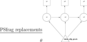
The general type of model considered in this thesis is a Bayesian hierarchical model (see Bernardo and Smith (1994) chapter 4). Hierarchical models have two or more levels of dependency. The hyperparameters θ specify the distribution of the latent parameters X which in turn specify the parameters of the likelihood functions for the data Y (this notation will remain consistent throughout). The hyperparameters themselves may in turn be modelled as random variables with a hyperprior.
The level of data is called the first level, the parameters of the likelihood are level two and so forth.
Normalisation of the posterior is one of the primary challenges to implementation of the Bayesian method. In recent years, the use of Markov Chain Monte Carlo (MCMC) methods has become almost ubiquitous in Bayesian statistical inference, due largely to the availability of cheap and powerful computing resources (Gelfand and Smith (1990)). One common algorithm for performing MCMC based inference is the Metropolis-Hastings rejection sampling algorithm.
Iterative Metropolis-Hastings algorithms (introduced in Metropolis et al. (1953) and generalised in Hastings (1970)) generate a Markov chain of samples from any target probability distribution (such as the posterior in Equation (2.4)). The samples of the Markov chain can then be used to form any desired summary of the target distribution. The desired distribution only needs to be known up to a proportionality constant and therefore the denominator in Equation (2.4) is not required.
A very simple summary is provided here; for details of the Metropolis-Hastings and
other MCMC algorithms, see Gilks et al. (1996). Suppose a target distribution has
density f X�. Then, given a sample value of Xt, a proposed value X� is generated from a
pre-specified proposal density qX�SXt� and then accepted with probability αXt,X��,
given by
X�. Then, given a sample value of Xt, a proposed value X� is generated from a
pre-specified proposal density qX�SXt� and then accepted with probability αXt,X��,
given by
 | (2.2) |
If the proposed value is accepted, the next sampled value Xt�1 is set to X�. Otherwise,
Xt�1 is set to Xt. If a symmetric proposal distribution is used (for example a random
walk or an independence sampler), then the q terms in Equation (2.2) cancel. Looping
over this procedure n times produces a Markov chain of samples X1,…Xn from fX�,
after convergence.
Constructing the algorithm is usually not difficult. Challenges are encountered when attempting to construct an algorithm that will return enough independent samples from the posterior to facilitate accurate inferences. MCMC methodology is plagued by the following issues.
In most practical problems a mixture of intuition, experience and ad hoc methods are used to determine the length of an MCMC run required to generate a sufficient sample from the posterior. This is particularly challenging for the forward stage of the palaeoclimate reconstruction project due to the non-parametric modelling approach which necessitates a very large number of highly correlated variables.
A directed acyclic graph, or DAG, is a powerful graphical tool for model building and illustration. A graph with directed arcs and no directed cycles is used to represent the model. The direction of the arcs gives the conditional dependencies.
Hierarchical models are most easily expressed using a DAG, where arrows between each variable denote dependence. If, for example, a variable a depends on another variable b in a statistical model, then the DAG for this is simply a � b.
Throughout this thesis, the structure of all models considered have an overall DAG corresponding to
 | (2.3) |
Each of the three levels may consist of multiple variables with extra dependency structure, suppressed in this simplified graph.
Bayesian inference procedures, such as those listed below, allow for inference on the distribution of the parameters given the data via Bayes rule:
 | (2.4) |
Bayesian Networks are probabilistic DAGs whose nodes represent random variables. The directed arcs of the DAG denote the conditional dependencies of the model represented. For example, Figure 2.1 shows a DAG for a hierarchical model;
It is common for the latent parameters to be modelled as a latent multivariate Gaussian field, particularly in spatial statistics (Banerjee et al. (2003), Finkenstdt et al. (2006)). This allows for a stochastic dependence between the latent parameters X to be incorporated into the model. One or more of the set of hyperparameters may be used to model the degree of covariance between these latent variables.
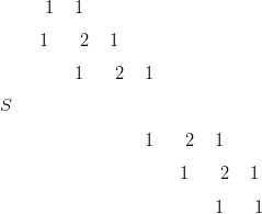
For a vector X defined in a discrete location space, a labeled graph G�V,ω� defines
the Markov structure of X. V��1,…,n� indexes the locations and ω is the set of edges
(dependency connections from one node to another) for each node of the graph. There is
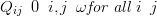
no edge between nodes i and j iff xi xjSx��i,j�.
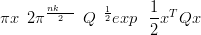
Definition 1 x ��x1,…,xn�T is a GMRF w.r.t. a labeled graph G�V,ω� with
mean μ and precision matrix Q iff its density has the form
 | (2.5) |
and
 | (2.6) |
Assigning a Markov structure to the latent field renders both the prior and posterior for the latent parameters to be a Gaussian Markov Random Field (GMRF) w.r.t. a graph G. The reason for using a Markov structure, as opposed to defining a variogram in continuous space, is for computational savings associated with the sparseness of the matrices required; see later in Section 4.1.
If the precision (inverse covariance) matrix for the latent field is sparse, then fast numerical algorithms may be employed; details of this are described in Section 4.1. These Gaussian Markov random fields model the response surfaces of previous sections as stochastically smooth across the location space.
If each node of the graph has an edge to all other nodes then the graph is said to be fully connected . Assigning a regular Markov structure to the graph breaks many of the edges resulting in a sparse precision matrix.
The use of Markov random fields requires the location space to be defined on a discrete grid. Use of a fine grid blurs the distinction between discrete and continuous space. The data for locations may then be shifted to the nearest gridpoint or left as continuous and calculations at these locations may be evaluated cheaply as weighted averages of the values at the surrounding gridpoint values.
Intrinsic GMRFs are defined by an improper log-density. No mean is specified and the the precision matrix cannot therefore be inverted to give the covariance matrix.
Intrinsic GMRF priors are often used for the parameters describing the latent surfaces. This allows for the specification of prior beliefs on the smoothness of the surfaces without specifying a prior mean.
Following Rue and Held (2005):
Definition 2 Let Q be a symmetric, positive semi-definite matrix with rank n�k A
0, where k A 0 is the dimension of the null space of Q. x ��x1,…,xn�T is an
improper GMRF of rank n�k A 0 with parameters μ,Q� if its improper density
is
 | (2.7) |
where SQSf is the generalized determinant of Q (the product of the non-zero eigenvalues).
Intrinsic GMRFs are improper; the precision matrices are not of full rank and cannot therefore be inverted to give a covariance matrix (see Rue and Held (2005) Chapter 3). In fact, the precision matrix for an intrinsic GMRF does not formally exist, however following Rue and Held (2005) the n�n matrix Q with rank n�k (and k A 0) is referred to as the precision matrix of the intrinsic GMRF.
An intrinsic GMRF of kth order is an improper GMRF of rank n�k, where PjQij � 0 for all i. Hence, the conditional mean of xi is the weighted mean of its neighbours, but has no specified overall level.
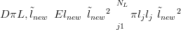
A convenient prior on a vector X whose indices are one dimensional may be derived from the random walk. For example, the first order random walk in one dimension is constructed from independent increments of X, defined on n discrete points (nodes on the graph G).
 | (2.8) |
which implies that
 | (2.9) |
for i @ j. The full, joint density for X is then derived from its n � 1 increments
(πx1Sx0�,…πxnSxn�1� where πxiSxi�1��Nxi�1,κ�1) given by Equation (2.8) as (again,
following Rue and Held (2005))
 | (2.11) |
Similar structure matrices may be constructed based on higher order random walks in any dimension of space, subject to edge effects. The imposition of a spatial structure models the latent surfaces as stochastically smooth using just a single hyperparameter κ. This hyperparameter controls the degree of spatial smoothing.
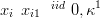
The parameters of many likelihood functions, particularly for counts data, require non-negative parameters. Link functions are therefore used to transform the unrestricted latent field variables into positive numbers.
For example, if the data are modelled as Poisson, then the rates (positive) may be modelled as the exponents of multivariate Gaussian distributed random variables.
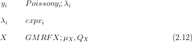
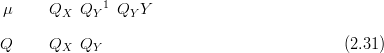
In this example the hyperparameters θ are comprised of the means and precisions of the latent field, μX and QX.
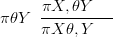
The Bayesian inference problem for models such as the one depicted graphically in Figure 2.1 is to infer posterior (i.e. given the data) probability distributions for the latent variables X and hyperparameters θ. i.e. to find
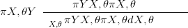 | (2.13) |
which is more conveniently expressed as
 | (2.14) |
The most common approach is to use MCMC to sample from the posterior for X and θ. This approach, while hugely popular, is not without its drawbacks (Sections 2.1.2 and 2.2.2). New techniques introduced in Rue and Held (2005) and developed further in Rue et al. (2008) offer a fast approximation called Integrated Nested Laplace Approximations (INLA).
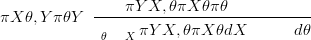
Starting with the identity
 | (2.15) |
Replacing the denominator with a normalised Gaussian approximation evaluated at
the mode (Xf θ�) yields
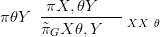 | (2.16) |
This is known as the Laplace approximation for the hyperparameters. The Gaussian
approximation for the latent field posterior,  GXSθ,Y �, is demonstrated in detail in
Section 4.1.
GXSθ,Y �, is demonstrated in detail in
Section 4.1.
The basic procedure for INLA type inference on Bayesian hierarchical models is as follows:
Full details of how this is achieved and the relative strengths and weaknesses of the method are examined in Section 4.1. It is sufficient here to note that implementation of these new methods is novel in the context of palaeoclimate research. They allow for increased sophistication in the forward model and more rigorous sensitivity analysis and model validation.
Contributions to the actual INLA methodology in this thesis consist of a method for performing fast updates to the entire posterior to correct for leaving out data; this has an immediate application in cross-validation in the inverse sense (see Section 2.6.2). Local corrections are sufficient for cross-validation in the forward sense as the location is known in this case.
Many counts datasets include zero-inflation; there are an excessive number of zero counts. Of particular interest is spatial data that exhibit such an overabundance of zeros. If these zero counts are ignored then information is lost. If zeros are modelled as arising in the same manner as the non-zero data, then statistical inference carried out on the dataset will be biased by them.
There are several methods for modelling data with many of these extra zeros that fall into three broad categories (see Ridout et al. (1998)):
The first technique, mixture models, accounts for zero-mean random effects. The parameters of the likelihoods for the counts are mixed with a distribution centred on zero. The resulting overdispersed likelihood will allow for some of the desired additional probability on zero counts, however, the variance will be increased and additional probability will also be placed on other counts far from the expected value.
Hurdle models (Mullahy (1986) a.k.a. two-part models Heilbron (1994)) provide for a two part likelihood. The first defines the probability of observing a zero count and the second part models only the positive counts. For example, if the positive counts are modelled using the zero-truncated Poisson then the count y is distributed as:
 | (2.17) |
where π0 is the probability of observing a zero count.
Unfortunately, the mean of the zero-truncated distribution is dependent on the form of the non-zeros probability. For example, if a Negative-Binomial distribution with the same mean as the above Poisson was truncated at zero then the means of the truncated distributions will differ. This inconsistency will compound any modelling errors and lead to biases in the inferences (Ridout et al. (1998)).
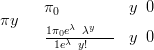
Zero-modified distributions are very similar to hurdle models; the key difference is that the zeros may still arise from the process that generates the positive counts as well as from a zero-only process. For example, the zero-inflated Poisson is given by
 | (2.18) |
where 1 � q is the probability of observing an essential zero count; i.e. a count arising from the process that generates only zero counts.
These are also referred to as structural zeros in the literature, with zeros arising from the process that also generates the positive counts referred to as non-essential zeros or sampling zeros .
This is equivalent to the Poisson hurdle model with π0 � 1 � q � qLikelihood0�.
However, this relationship will of course vary with the choice of non-zero-inflated
distribution.
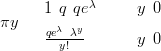
The general form for a zero-modified counts distribution is
 | (2.19) |
where L is the counts likelihood for the non-zero-inflated version of the distribution. It is a mixture of the non-zero-inflated likelihood and a point mass at zero.
These latter are the most flexible class of distributions for modelling zero-inflated counts data and they are the focus of the work presented here; this is because the pollen data are most accurately described by the mixture of a point mass at zero and a counts likelihood that may still return a zero. The term zero-inflated will be reserved for this method of modelling extra zeros from here on.
A zero-inflated distribution of counts has an extra parameter over the non-zero-inflated version. For spatial problems, modelled non-parametrically, this doubles an already large number of parameters in the model. As computational overhead is already one of the main challenges to Bayesian analysis of such models, it is desirable to reduce the number of free parameters.
If the parameter governing the point mass at zero and a parameter of the not strictly zero counts part (e.g. the mean) are related, then a more parsimonious model may reduce the number of parameters in the spatial model by half.
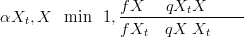
In the context of hurdle models, Heilbron (1994) calls this a compatible model . An analagous model for a zero-inflated Poisson is introduced by Lambert (1992), wherein the log of the Poisson rate is modelled as
 | (2.20) |
for some covariate matrix B. The probability of an essential zero and is given by
 | (2.21) |
Lambert advocates such a model based on the absence of prior information about the relationship between the two variables. Lambert proposes the use of such models when the covariates affecting the two variables are the same.
Salter-Townshend and Haslett (2006) showed that using such a functional link in such models not only reduces the number of parameters by half, but that in the context of spatial data analysis ignoring such relationships, if they exist, may lead to a substantive loss in accuracy of inference. In that paper, the “probability of potential presence” q is modelled as being equal to the Binomial parameter for zero-inflated Binomially distributed counts.
A more flexible model may be readily achieved through the addition of a single extra parameter α. A power law functional relationship such as
 | (2.22) |
with α A 0 provides a simple and intuitive, yet flexible model. This is the zero-inflation model that is used for the remainder of the thesis.
If dealing with rates λ rather than proportions, a relationship based on a
transformation of the rates to the �0,1� interval is required, such as q � α
α
This is related to Lambert (1992)’s model; solving for q in Equations (2.20) and (2.21) gives
 | (2.23) |
Equation (2.22) is monotonic for positive α; an increase in p implies an increase in q. This has the effect of limiting the model with the constraint that as the rate or proportion increases, the probability of observing an extra zero decreases. This flexible yet simple model is one of the lesser contributions of the work described in this thesis. Of course, this model should only be applied to data which exhibit such a relationship or when such a feature is desirable in the model. Justification for this model for the motivating pollen and climate dataset is given in Chapter 6 and so this is the model used in the rest of the thesis.
As per Section 2.1, inverse regression may either mean regressing cause on effect directly (referred to here as classical inverse methods) or regressing effect on cause (the forward model) and then inverting the model to provide estimates of cause given effect. The latter is the approach taken here; response surfaces are fitted using modern data on climate and pollen assemblage pairs. This calibrated model is then inverted to predict (or reconstruct) climate given an assemblage for which there is no climatic data.
One important aspect of palaeoclimate reconstruction is the fitting and use of response surfaces (Bartlein et al. (1986), Huntley (1993) and Allen et al. (2000)). The essential issues in the Bayesian modelling of these are presented in terms of a simple hierarchical model. The random variation in the observations (that is, the likelihood) is Gaussian, and all precision parameters are taken to be known. For illustration purposes a simple toy model is presented. Initially in this chapter a univariate model is used, subsequently generalising to multivariate cases. In later chapters, assumptions such as known precisions, are relaxed. The distinction between the forward and inverse stages (see Section 1.1) is stated and illustrated. The procedure is critically analysed and an inverse performance metric is introduced.
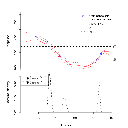
The basic idea is presented in Figure 2.2. Pollen counts Ỹ ��ỹj;j � 1,…,10� on a single
plant taxon are available at 10 regularly spaced points having known climates  ��
�� j�. A
model is fitted to these training data, represented by the smooth red line with
associated uncertainty interval (dashed red line); this is the forward stage. It
models the response of a single taxon to changes in one-dimensional climate. Note
that response is measured indirectly; it is a latent variable. In the context of
the pollen data, response is the propensity to produce pollen, as a function of
climate.
j�. A
model is fitted to these training data, represented by the smooth red line with
associated uncertainty interval (dashed red line); this is the forward stage. It
models the response of a single taxon to changes in one-dimensional climate. Note
that response is measured indirectly; it is a latent variable. In the context of
the pollen data, response is the propensity to produce pollen, as a function of
climate.
A new count ỹnew is introduced and inferences are made on the associated unobserved climate lnew; this is the inverse stage. The figure presents two examples of ỹnew. The model adopted is such that for one of these the inference on lnew is represented by a unimodal density and for the other the density is bimodal. This potential mutlimodality is a consequence of the non-monotonic shape of the response surface.
|
|
The forward fitting stage is a form of non-parametric regression, in which the only requirement is that the response surface is smooth. A Bayesian approach involving a Gaussian process prior is implemented. In Section 2.5.2 a simple example is used to present the details. These are trivial if, as assumed there, the variance parameters are known and the likelihoods are Gaussian. The inverse stage, even for this toy model, is not trivial. Nevertheless, for this model, with known parameters, it is simple to compute.
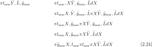
This is formalised as follows, for each new count, where the Gaussian random function
XL� models the response surface:
There are a number of interesting features of such a problem, many of which are not immediately obvious. These are most usefully demonstrated via investigation of an example toy problem, which is simple yet similar in spirit to the palaeoclimate reconstruction problem. This also serves to introduce some modelling choices which are retained throughout much of this thesis.
Counts data Ỹ are available at Nd locations  . The response X � XL� is unobserved and
treated here as a random function, defined on a fine regular grid L� of 100 points across
the location space. The interest here is its conditional distribution given the training data.
The Bayesian formulation of the problem is then
. The response X � XL� is unobserved and
treated here as a random function, defined on a fine regular grid L� of 100 points across
the location space. The interest here is its conditional distribution given the training data.
The Bayesian formulation of the problem is then
 | (2.25) |
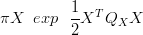
where X is the latent response and K is the normalising constant. The data are
conditionally independent, given the latent surface. In such Bayesian approaches K is
source of much technical difficulty, even when πX� is Gaussian. However when the
likelihood is also Gaussian, as here, K is available analytically. For this example, the
surface Xl� is the likelihood mean at l > L and σY 2 is the variance. The prior πX� and
the likelihood πỸSX, � are thus conjugate, leading to a Gaussian posterior,
provided the prior and likelihood precision matrices, QX and QY respectively, are
known.
� are thus conjugate, leading to a Gaussian posterior,
provided the prior and likelihood precision matrices, QX and QY respectively, are
known.
Across all gridpoints L� in the location space, the likelihood contributes
 | (2.26) |
where
 | (2.27) |
and the likelihood precision matrix QY is diagonal and of dimension NL �NL, where NL is the number of gridpoints. The diagonal entries are:
 | (2.28) |
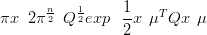
The prior on X is an intrinsic Gaussian Markov random field (GMRF), given by
 | (2.29) |
with the precision matrix QX given by
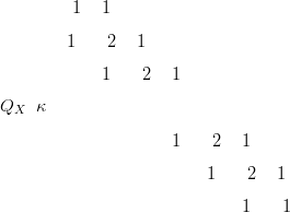 | (2.30) |
The model has two scalar parameters; the positive scalar prior precision parameter κ
and the likelihood variance σY 2. The higher the κ value used, the greater the smoothness
of the latent surface XL�. The decision to model the surface on a regular grid
rather than specifying a continuous model defined at the datapoints is due to the
desirable properties of GMRFs as discussed in Section 4.1 and is not discussed
here.
The Markov property is inherited by the posterior which is a multivariate Gaussian with mean and precision matrix given by
Using this analytical form for the posterior of the latent surface given the data, the
inverse stage posterior of Equation (2.24) may be computed numerically. The locations
are discrete so the posterior for unknown location given a new count is defined only on a
finite number of possible gridpoints. The posterior is therefore a probability mass
function and normalisation is provided by rescaling the unnormalised product
of the prior and likelihood functions such that the total is unity. A uniform
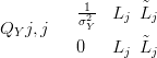
prior  is imposed here and the likelihood of the new count ỹnew at any given
location L is NXL�,σY 2�. The integral over the unidimensional latent surface is
performed analytically. Sample calculations are provided in Table 2.1 for a given
ỹnew.
is imposed here and the likelihood of the new count ỹnew at any given
location L is NXL�,σY 2�. The integral over the unidimensional latent surface is
performed analytically. Sample calculations are provided in Table 2.1 for a given
ỹnew.
|
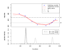
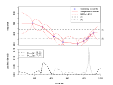
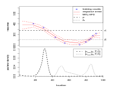
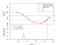
The model parameters κ and σY 2 effect the forward and therefore the inverse stage results. Inferences on the same dataset as in Figure 2.2, but using different values of κ and σY 2 are presented in Figure 2.3.
|
Figure 2.3 illustrates the effect of varying the model parameters κ and σY 2. Comparisons with the parameters used and results obtained for Figure 2.2 are made here. In Figure 2.3(a), κ is an order of magnitude larger. This induces a greater degree of smoothness in the latent surface and tightens the bounds of the 95% highest posterior density (HPD) region of the forward stage.
In Figure 2.3(b) κ is an order of magnitude smaller. The surface parameters linearly interpolate the data and uncertainty is high away from the datapoints. This leads to a highly multimodal posterior for the inverse stage. As κ goes to zero (no smoothing), the forward stage posterior tends toward the likelihood. The forward model then informs only at the datapoints and the inverse stage will yield a uniform mass function for new counts not close to training data counts. For new counts close to one or more training counts, the inverse stage posterior will be spiked at the associated training data locations.
In Figure 2.3(c) σY 2 is an order of magnitude larger. The likelihood density has a larger spread, as does the forward stage posterior. The prior on X begins to dominate the posterior for X. The inverse stage posterior then has a larger variance and the amplitude of the minor mode associated with y2 grows relative to the major mode. As σY 2 increases, the inverse stage posterior flattens out.
In Figure 2.3(d) σY 2 is an order of magnitude smaller. As there is more data on the
major mode of the posterior for location given y2, this serves to increase that mode;
consequently, the minor mode is reduced. As σY 2 decreases, the forward stage posterior
becomes dominated by the likelihood at the datapoints. Away from the datapoints, the
prior dominates. Inferences on new counts that are close to training data counts will have
inverse stage posteriors with sharp peaks at the associated training data locations,
 .
.
MCMC is the dominant technique for Bayesian inference; as discussed in Section 2.2.2, the main crux of this methodology is computation. Cross-validation is a common technique for assessing the model fit to data. This requires re-fitting the same model for many subsets of the dataset in order to form reference distributions for the left out points. Model evaluation by cross-validation is very unsuited to the brute force approach of simply conducting many MCMC re-runs.
Model evaluation techniques in Bayesian problems are a well documented research area. However, Bhattacharya (2004) observes that “there seems to be no literature in this context [model assessment in inverse problems]”. As stated previously, inverse problems refers to studies in which the forward model (cause implies effect; input drives output) is inverted, with the objective of predicting (or reconstructing) input given output.
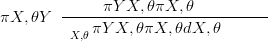
Ultimately, the objective of the investigation is to make accurate inferences on unobserved
climates given fossil counts. Therefore, the performance metrics introduced below focus on
the inverse stage of the problem. Pairs of ‘new’ data ỹnew, new� are generated and the
ability of the model to predict
new� are generated and the
ability of the model to predict  new given Ỹ,
 � pairs and ỹnew is evaluated.
The predictive distribution here is simply the posterior for the inverse stage,
πlnew �
� pairs and ỹnew is evaluated.
The predictive distribution here is simply the posterior for the inverse stage,
πlnew � newSỸ,
 ,ỹnew�� πlnewSdata�. The performance is summarised by a statistic on a
function of the inverse stage posterior πlnewSỸ,
,ỹnew�� πlnewSdata�. The performance is summarised by a statistic on a
function of the inverse stage posterior πlnewSỸ, ,ỹnew� and the ‘unobserved’ location
 new. As the posterior for location is often multimodal and seldom symmetric, simple
statistics such as the distance between the modal prediction and
new. As the posterior for location is often multimodal and seldom symmetric, simple
statistics such as the distance between the modal prediction and  new will be
insufficient.
new will be
insufficient.
For ease of notation, πlnewSdata� is denoted πL�. The desirable properties of the
performance metric D � DπL�, new� are listed here.
 D � 0
D � 0
One such metric is the expectation of the square of the difference between the new
location  new and the predicted location under the posterior for the inverse stage given the
new count ỹnew. For a location space discretised into NL gridpoints, this is readily
computed as
new and the predicted location under the posterior for the inverse stage given the
new count ỹnew. For a location space discretised into NL gridpoints, this is readily
computed as
 | (2.32) |
where SSlnew � newSS is the distance between lnew and
  new. D is then the mean-squared
error of prediction.
new. D is then the mean-squared
error of prediction.
If the location space is rescaled to lie between 0 and 1 then this metric will lie between
between 0 and 1 (or 0 and  2� for 2-dimensional location space).
 | (2.33) |
 | (2.34) |
This metric will tend to unity as the predictive probability mass function tends
to unity at the greatest distance in the location space from  new and will tend
to zero as the predictive probability mass function tends to unity exactly at
new and will tend
to zero as the predictive probability mass function tends to unity exactly at
 new.
new.
Measurement of predictive performance is closely related to cross-validation of the model
using the training dataset. In leave one-out-cross-validation, the ability of the model to
predict each  i (rather than a new point), given the remainder of the training data
Ỹ,�
i (rather than a new point), given the remainder of the training data
Ỹ,� j(i;j � 1,…,Nd�� is assessed. This step is repeated for each datum and
a discrepancy measure summarises the validity of the initial analysis. This is
in fact cross-validation for the inverse problem, which is discussed in detail in
Section 4.2.
j(i;j � 1,…,Nd�� is assessed. This step is repeated for each datum and
a discrepancy measure summarises the validity of the initial analysis. This is
in fact cross-validation for the inverse problem, which is discussed in detail in
Section 4.2.
One method for speeding up the brute force approach of repeated MCMC samplers is the use of importance sampling. The “saturated posterior” refers to the model trained on all of the modern data. As leaving out a single point will only have a small effect on this distribution, the proposal density for a new MCMC run uses the saturated posterior as an importance sampler. The importance weights are easily calculable for the forward problem as they are proportional to the correct posterior to saturated posterior ratio. This ratio, having the same prior and likelihood terms, is expressible as the inverse of univariate likelihood of the left out datum, given the sample parameters (see, for example, Gelfand (1996)).
Cross-validation in the inverse sense is a more difficult challenge. The importance weights now typically involve an intractable integration (see Section 4.2 for details). In the inverse case, a prior for the input must also be constructed. This complicates the analysis.
Being the first attempt to address the issue of cross-validation in inverse problems and its applications to model assessment, Bhattacharya and Haslett (2008) provides an important benchmark. In that work, the authors use importance resampling (advocating without replacement) to approximate the posterior distribution of the parameters and a pre-chosen datum given the data minus the left-out datum. The importance weights are quick to compute and proposal densities are constructed to maximize the efficiency of the predictive distribution MCMC sampler. This technique is referred to as Importance Re-sampling MCMC (IRMCMC) for (leave-one-out) cross-validation in inverse problems. The difference between this resampling approach and the forward problem importance sampling is that for the first MCMC run, a selected datapoint is left out and regarded as a random variable. The integrations in the calculation of the importance weights for the resampling stage are no longer intractable. This observation is the key to the procedure (see Section 4.2.2).
An efficient sampling algorithm is thus constructed for the cross-validation. However, multiple sampling runs are still required. Bhattacharya and Haslett (2008) presents an example where brute force MCMC re-runs for each of 62 data sample sites takes 16 hours. IRMCMC achieves comparable, if not better, results in less than 40 minutes. For the example in Haslett et al. (2006), brute-force MCMC replications would take many years.
A new method for cross-validation in the inverse sense is presented and developed in Section 4.2. Essentially, fast alterations are made to the saturated posterior for the forward model to correct for left out data. As the locations (inputs) are already made to lie on a finite grid, the marginal likelihood may be computed for all possible values of the left out point; thus MCMC is entirely avoided.
In Chapter 6 it is demonstrated that cross-validation in the inverse sense for this same problem is thereby reduced to less than 1 hour using the techniques presented in this thesis that synergize with the INLA method. In fact, that run-time is for a superset of the data with a more sophisticated hierarchical model and formal estimation of several hyperparameters that were necessarily preset ad-hoc in previous MCMC / IRMCMC attempts.
Palaeoclimate reconstruction is an example of an inverse problem. Existing attempts to infer climates from ecological data involve a trade off between model complexity and speed of inference. The Bayesian framework is preferred due to its ability to honestly model uncertainty by treating unknown parameters as random variables. This is particularly important when inverting forward models to obtain the inverse posteriors.
Sampling based methods, such as MCMC, are the standard methodology in Bayesian inference. Non-parametric models, with high numbers of random variables, may be poorly suited to these computationally intensive methods. Inference is labourious and this negatively impacts the level of complexity of the models. Fast, approximate methods for performing Bayesian inference allows the development of more sophisticated models for the palaeoclimate reconstruction problem. These include, for example, zero-inflated models.
Model comparison and validation, requiring many similar versions of the same models, is an important aspect of any statistical study. Validation of inverse problems occupies only a limited literature. MCMC type inference is unsuitable to this challenge. Existing approximate inference techniques must be extended to meet this challenge. Conversely, the palaeoclimate problem presents an interesting and challenging test of the approximate inference methodology.
Since the “proof of concept” paper Haslett et al. (2006), the work contained in this thesis to modelling the RS10 dataset may be summarised as follows: