The motivating problem is palaeoclimate reconstruction from pollen data. This chapter applies methods and models established in earlier chapters to this problem. No fossil reconstructions are presented; the focus here is in model fit and validation of the inverse problem. The inverse problem here is to predict (reconstruct) climate variables given a pollen assemblage.
Models are evaluated using cross-validation of the modern dataset in the inverse sense and the use of the inference-via-marginals approximation is evaluated. The inverse cross-validation is achieved using the fast updates derived in Section 4.2.3. The nested model is novel in this application.
The work contributed by this thesis to the ongoing Bayesian palaeoclimate reconstruction project described in Haslett et al. (2006) is presented. The main crux of the methodology up to and including the publication of that paper was acknowledged to be computational. Approximation of the posterior for the parameters of the forward model with closed form expressions via INLA greatly reduces the computations (Section 4.1).
The dataset comprises 28 pollen taxa proportions. There are 7742 sampling locations in the modern training dataset, each of which has physical variables (longitude, latitude and altitude) and climate recorded. The climate is measured here as the growing degree days above 5oC, GDD5 and the mean temperature of the coldest month, MTCO. The former is a temperature sum and is a measure of the growing season.
The data are reported as counts, with total equal to around 400. In fact, many of the sampling locations do not have the total count reported; only the proportions are reported. In these cases, the somewhat unsatisfactory step of assuming a total count of 400 is taken. The reported climates are typically not in fact from precisely the same location in physical space as the lake from which the pollen grains are taken. The nearest meteorological station provides data on the climate. Thus an error term should be appended to these climatic observations. Expert opinion is used to inform these and a post-hoc method for correcting the inverse predictive distributions is used in Section 6.4.3.
The ultimate goal is to reconstruct these climate variables given fossil pollen counts. As this task cannot be assessed directly, inverse cross-validation on the modern training data, for which climate is known, is presented as a best-available model validation tool. This task could only be performed approximately in Haslett et al. (2006); the MCMC methodology was too labourious to cope with re-fitting the model for each left-out datum. The saturated posterior was therefore re-used for each approximate cross-validation step.
The INLA methodology allows approximations to be fitted quickly to the posteriors for the response surfaces and assorted hyperparameters, given the counts data. This thesis presents one of the first large scale tests of the INLA technique. The RS10 dataset is not only large, but some details present extra challenge to the INLA method that are not addressed in Rue et al. (2008): There are multiple, potentially interacting, counts at each sampling location; each of these are subject to overdispersion and zero-inflation relative to standard counts likelihood models. The counts vectors are constrained by the data collection method (count until a pre-chosen total is sorted) and are thus compositional in nature. The climate space should in fact be 3D; although alluded to in Rue et al. (2008), large scale problems such as this pose problems for the INLA methodology.
Although additional assumptions and / or approximations have to be made to allow the application of INLA type inference to the dataset, the method performs well. Running times to fit the forward model approximations are around 4 orders of magnitude faster than for MCMC based inference. This is on a 50 � 50 size grid across 2D climate space; each non-parametric response surface is thus described by a latent field of 2500 random variables. Leave-one-out cross-validation for the inverse problem is achieved using fast updates to the saturated posterior in around an hour. The approximations’ most appealing characteristic is the closed form expressions for the posterior distributions; this allows such manipulations as the fast updates of posterior moments used for inverse cross-validation.
Application of these methods to the RS10 pollen dataset does, however, reveal some drawbacks to the INLA method:
The time taken to fit a GMRF approximation to the response surface of a single taxon on a 50 � 50 2D grid is of the order of 30 seconds for a 50 � 50 size grid on the climate space. Finding the modal value for the hyperparameters takes about 2 minutes for a model with 3 hyperparameters (for each iteration of the search for the modal configuration, a full GMRF approximation to the parameters given the data and the hyperparameters must be fitted). Exploration of the 3D grid of hyperparameters takes up to 5 minutes.
In all cases, the GMRFLib C library was used. This library of C functions is
available as a free download at http://www.math.ntnu.no/~hrue/GMRFLib/
Other freely available C libraries used were GSL, LAPACK, BLAS, an ATLAS. The free
statistical software language R was used for post-processing results and for creating all
images and plots appearing in this thesis.
The hardware used is a dedicated Beowulf Linux cluster, consisting of 3 machines each of which has 2 3.4GHz processors and 4GB of RAM. This allows for the parallel implementation of the INLA method on up to 6 taxa at a time. Running the code on a single node machine of similar speed as the cluster nodes (such as a laptop or PC) involves running each INLA fit sequentially. Thus run times are increased approximately 5-fold for the 28 taxa dataset when parallel resources are not available (6 processors handle 6 taxa at a time; this requires 5 such groups of 6 for the 28 taxa problem). As all models considered disjoint-decompose, no message passing between nodes is necessary. The algorithms are perfectly parallelizable and specialist parallel computing code is not strictly required.
The methodology for the pollen dataset in Haslett et al. (2006) suffers from the usual issues related to MCMC based inference. Mixing is poor and convergence is far from assured, even for runs lasting several weeks on multiple machines. Cross-validation, requiring many re-runs, is therefore all but impossible; for this reason the model validation results obtained here using the INLA method are not contrasted with MCMC based cross-validations.
Although the model in Haslett et al. (2006) appears to perform joint inference of all plant taxa at once, the underlying Dirichlet prior has an implied independence structure, given the constraint. Had inference been performed on each taxon separately and the results scaled post-hoc, the outcome would have been identical.
In the forward problem, the responses are modelled a-priori as independent GMRFs, via an appropriate link function to the ���,�� range. Two models are considered in this chapter; a model that is disjoint-decomposed by taxon (referred to as the by-taxon marginals model) and a nested model. A grid size of 50 � 50 was used to model the GMRFs. The granularity of this grid was selected based on expert opinion of the measurement accuracy of the reported climates.
The forward model for each taxon is fitted independently of the others. Inversion of the model (for cross-validation) is also performed separately for each taxon, with scaling to induce the constraint (see Section 3.5.2) performed via Monte-Carlo. The joint predictive distributions are then formed as the normalised product all 28 taxon-specific inverse predictive distributions.
For all models in this chapter, the prior on the latent field is an intrinsic GMRF. The prior is specified through the precision matrix, which has a second order Markov structure matrix S given by
|
| (6.1) |
where d2 i,j��ir �jr�2 �ic �jc�2 is the squared distance between node i and node j on
the 2D discrete grid. The subscripts r and c stand for the row index and column index of
a node on the 2D grid.
i,j��ir �jr�2 �ic �jc�2 is the squared distance between node i and node j on
the 2D discrete grid. The subscripts r and c stand for the row index and column index of
a node on the 2D grid.
This is the precision matrix derived from a second-order random walk in 2-dimensions that appears in Rue and Held (2005). (Appropriate corrections for the boundaries are made so that the rank of the matrix is N � 2, where N � 50 � 50; these appear in Kneib (2006)).
The prior precision matrix Q is then the structure matrix S scaled by the positive hyperparameter κ
 | (6.2) |
The second order Markov structure ensures a stochastically smooth response surface with higher κ values for smoother surfaces.
Unless otherwise specified, all likelihood models are zero-inflated and overdispersed. Furthermore, all counts likelihoods are overdispersed Poisson (Negative-Binomial) or overdispersed Binomial (Beta-Binomial). Where required, the normalisation of the product-of-Poissons type models is performed via Monte-Carlo sampling as per Section 3.5.7.
A maximum of three hyperparameters are included in the model for each taxon:
Models with non zero-inflated likelihoods have only the first two hyperparameters.
Fitting of the forward model is performed using the INLA methodology. A GMRF approximation for the saturated posterior of the transformed latent surfaces is made. The Laplace approximation for the hyperparameters is used; however they are then fixed at their posterior modal values, for simplicity. This results in a large computational saving, with seemingly no substantive loss in accuracy (see Section 6.4.1).
To summarise, the goal is to build closed-form posteriors on latent random variables
X, which describe response-to-climate surfaces for all plant taxa. i.e. the posterior
πXSY,L� is sought. There are NT counts Y associated with locations in the climate
space L. A-priori, the X are modelled as independent across the NT taxa and
stochastically smooth across discretized L via intrinsic GMRF specification.
The posterior is found approximately using the INLA methodology detailed in
Section 4.1.
The independence is due to the disjoint-decomposition; this is first done taxon-by-taxon and the results are shown to have an error associated with this decomposition, using the methods developed in Section 5.3. A nested compositional model, as introduced in Section 5.3.2 is then invoked to reduce this error. This involves a re-ordering and scaling of the data, with inference then proceeding as per the by-taxon model.
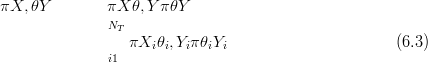
Thus, the goal is to fit the decomposed forward model to the modern data Y
where the right hand side is fitted using the INLA method. Thus, given GMRF priors
on πXiSθi� and univariate, zero-inflated counts likelihoods πyi,jSxi,j,θi�, the by-taxon
posteriors are formed
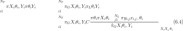
with subscript G denoting the GMRF approximation and subscript L denoting the
laplace approximation. The constant C is determined by normalisation on the
grid upon which the πLθiSY i� are defined (see Section 4.1.3). NL is the total
number of locations in L at which there are data. πGXiSθi,Y i� are formed as per
Section (4.1.1).
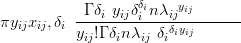
All likelihoods in the by-taxon model are zero-inflated Negative-Binomials:
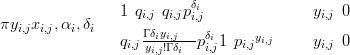 | (6.5) |
where the parameters αi and δi are part of θi, pi,j � and qi,j �
 αi
αi
For those modules in the nested compositonal model that have only one other term in the same nest zero-inflated Beta-Binomial likelihoods are employed:
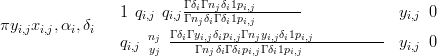 | (6.6) |
with pi,j � , qi,j �
 αi and nj is the total count at location j. All other
likelihoods in the nested compositional model are zero-inflated Negative-Binomials, as per
Equation (6.5) above.
αi and nj is the total count at location j. All other
likelihoods in the nested compositional model are zero-inflated Negative-Binomials, as per
Equation (6.5) above.
Fast updates to the saturated posteriors in Equation (6.3) using the method developed in Section 4.2.3 delivers a method for inverse leave-one-out cross-validation without recourse to re-fitting the model with one less datapoint. Inversion of these leave-one-out posteriors is straightforward due to the discretization of L to a lattice.
The Δ statistic (percentage of points lying outside their leave-one-out cross-validation inverse predictive distribution 95% highest posterior distribution region) is computed across all training data and all taxa. Values much larger than 5% indicate a poor model fit to the data.
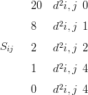
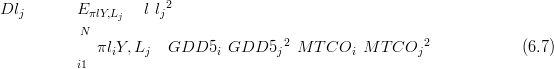
The sample density and mean value for Dlj� (the expected squared distance to the
observed climate lj, under cross-validation) are used to compare models. This is a
summary statistic (introduced in Section 2.6.1) on the predictive precision of the model
in the inverse problem. In a 2D climate space across GDD5 and MTCO, the D metric
for climate lj ��GDD5j,MTCOj� is given by
Inversion of the forward model was performed in Haslett et al. (2006) using MCMC. One-at-a-time sampling based inference of the inverse problem may be avoided altogether when the climates are constrained to lie on a discrete grid. The GMRF approximation in Section 4.1.1 already requires the use of such a grid. The posterior predictive probability mass function for the inverse problem is calculated at all discrete points on the grid and hence may be normalised.
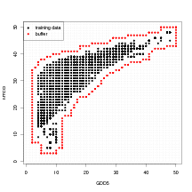
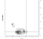
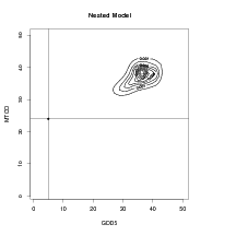
In order to speed up the numerical inverse predictive distribution algorithm, those points lying outside a region of support were eliminated from the computation. This is possible as the modern training data all lie within a zone defined as the observed modern climate space. Although, theoretically at least, prehistoric climates may have occurred that were outside this zone they are not of interest as the response surface method requires that the palaeoclimates have some modern analogue. The zone, with buffer, is shown in Figure 6.1 for a 50�50 regular grid. Use of this buffer zone is equivalent to placing a prior of zero on points outside the buffer and a uniform prior inside for the inverse predictive distributions.
The response surfaces interpolate / extrapolate the counts data, but only within this bounded region. Areas outside this buffer zone are deemed to be outside the support of the data and are not considered. All internal points are interpolated.
Many of the counts / proportions data are exactly zero. For the 28 plant taxon dataset a full 63.16% of the modern counts are zero. The data is highly zero-inflated and models not accounting for this will underestimate the expected proportions (see Salter-Townshend and Haslett (2006)).
Zero-modified distributions (Section 2.4.1) provide a way to account for these additional zeros explicitly in the model. However, the zero-modified distribution has two parameters; to facilitate compatibility with the GMRF approximation of Section 4.1.1, likelihoods must be functions of a single parameter.
Models of the type introduced in Salter-Townshend and Haslett (2006) and Section 2.4.1 provide a solution to this problem; in fact this type of model was motivated by the pollen dataset and was developed as a single-process model before compatibility with the GMRF approximation was considered. This model does not apply to every zero-inflated dataset; it was motivated by analysis of the pollen dataset specifically and applies to any dataset in which the probability of potential presence and the abundance when present are governed by a single latent process.
The motivation for using Equation (2.22) in the pollen data analysis is based on logical conclusions on the nature of ecological counts data. Martin et al. (2005) identify four sources of zeros in observation of counts data in ecological datasets: the first two are essential / structural zeros, which they refer to as “true zeros” and the last two are sources of non-essential / sampling zeros which they refer to as “false zeros”.
The four sources in Martin et al. (2005) are:
Applying the four sources of zero count identified by Martin et al. (2005) to the RS10 pollen dataset informs a model for the extra zeros.
Modelling the data with the response surface technique (Section 2.5.1) shows the first source to occur when the response tends to zero. Therefore this source will be accounted for by any response surface model where the response tends to zero in areas of unsuitable climatic conditions. The second source is due to non-climatic (and unmeasurable) factors, such as plant migration, soil type and topology. The third source is a factor of the finite size of the sample; the plant taxon is present in the location of the sample, but not in the sample itself.
The second and third sources become one and the same (from a climatic viewpoint) if there is a uniform pollen rain in regions where the plant taxon occurs. This is one of the principles of pollen analysis introduced in Birks and Birks (1980) and is due to atmospheric turbulence mixing the pollen and spores (see also Smol et al. (2001)). This single source of extra zero is then referred to as the non-climatic source and is the primary concern here.
The final source of zero count is accounted for by the counts likelihood function. For example, using a Binomial likelihood for the counts, given there are no zeros arising from sources one to three, will deliver this final source of zero. These are effectively non-extra zeros and as such are part of the non-zero-inflated model.
Therefore, a zero-inflated model is required to account for a single source of extra zeros, the non-climatic source. The single-process model in Section 2.4.1 is advocated for the pollen and climate dataset. The justification for such an approach is that the environmental pressure exerted by climate influences the probability of presence and the expected proportion if present in a related fashion.
This is not to say the two are the same; all that is required to justify the single-process zero-inflated model is that a single process governs both presence and abundance when present. This is the case if the random extra zeros due to non-climatic factors are more likely to occur in regions where the climate is less suitable. This follows as a natural assumption; non-climatic factors promoting absence (such as unsuitable soil type) will be more likely to cause a plant type to fail in climatic regions where the plant is already struggling than in conditions under which it thrives.
The power link in Equation (2.22) is motivated for the pollen dataset by several simple observations:
 | (6.8) |
 | (6.9) |
The simplest functional relationship between the response and the probability of potential presence is that q is some power of r. Limiting this power to to be positive ensures that q increases monotonically with r (see Section 2.4.1).
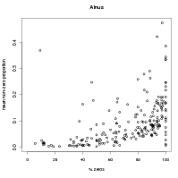
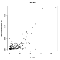
The validity of this simple, monotonic relationship between probability of potential presence and abundance when present is demonstrated in Figure 6.2. Plots such as these suggest a positive relationship between probability of potential presence and abundance when present.
|
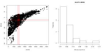
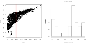
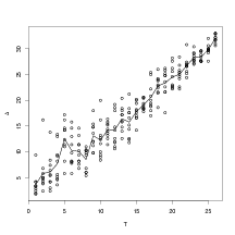
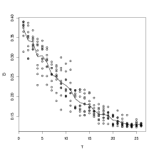
Further evidence from the data that the power-law monotonic relationship between probability of potential presence and abundance when present is given by Figure 6.3. Neither probability of potential presence or abundance when present are directly estimable from the data. However, the probability of non-zero proportion and the positive abundances act as crude proxies for these values. These proxies are plotted in Figure 6.3.
|
There are three hyperparameters specified in the model for pollen response to climate. These are; (i) the smoothness of the response across climate space, (ii) an overdispersion parameter and (iii) the power index for the zero-inflation. In order to integrate out the hyperparameters, the model is fitted for each discrete triplet and a weighted average is calculated, as per Equation (4.22).
Computation time and memory usage are of real concern in performing the cross-validation. Evaluating the inverse predictive distributions only at the modal value of the posterior for the hyperparameters reduces both run-time and memory usage by a factor of the number of discrete triplets. Even a coarse grid across the hyperparameter space results in an average of 54 for the number possible configurations of the three hyperparameter values for each taxon.
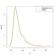
Evaluation at the mode represents an approximation to the integration over the hyperparameters. The data are not overly sensitive to the hyperparameters as they depend on them indirectly. However, an evaluation on the impact of using the model fitted at the modal hyperparameters (modal-hyperparameters approximation) must be conducted to justify the saving in computation.
Figure 6.4 shows the effect on the predictive power in the inverse sense for a model evaluated using the modal hyperparameters and the same model having integrated out the hyperparameters (the model used is that in Section 6.4.5). The predictive power of a model is summarised using the performance statistic introduced in Section 2.6.1. The expected squared distance to the true left-out observation is calculated, with expectation taken w.r.t. the posterior predictive inverse cross-validation distribution. The kernel density estimate of the expected squared distance D to the left-out observation lj (climate) appears to be insensitive to the use of the modal-hyperparameters approximation. This result, along with the large computational saving of about two orders of magnitude, justifies the use of the modal-hyperparameters approximation.
|
|
Inference using the decomposed by-taxon model was applied to the pollen dataset. Under the marginals model (Section 3.2.1) each taxon is taken as independent of all the others. The individual taxa returned cross-validation Δ statistics that were consistent with theory; i.e. about 5% of points fell outside their 95% highest predictive distribution region (see Figure 6.5).
|
|
The mean value of Δ is 4.15% (see Figure 6.5). This is around the theoretical value of 5% or less, given a model that fits the data (see Section 5.3.1).
However, bringing the cross-validation predictive densities for all taxa together
reveals an error. For 2 taxa there are �28
2 �� 378 possible choices of 2 taxa; for 3
taxa there are �28
3 �� 3276 unique combinations; etc. Taking a random 10 of
these �28
T � possible combinations for each of T ��1,…27� and computing the
ΔT� statistic for each gives an indication of the relationship between T and
Δ.
If the joint model (all taxa) disjoint-decomposes exactly, then ΔT� should stay
around 5% (while DT� goes down). This is clearly not the case, as shown in
Figure 6.6. Δ increases with T, showing that the plant taxa are not conditionally
independent given climate. Thus the joint model does not disjoint-decompose exactly.
Figure 5.1 indicates that this occurs when the response surfaces are correlated, given
climate.
|
|
The ΔT� plot in Figure 6.6 clearly demonstrates that the disjoint-decomposition of the
model by taxon is not a good fit to the data as error rate increases with the more taxa
modelled. Even still, the inverse predictive power of this model as measured with D
increases with increased T. This result is shown in Figure 6.7. D (the expected squared
distance to the observed normalised climate) decreases as T increases. It shows that as
more taxa are modelled, the precision of the inverse predictive densities becomes higher.
This relationship is not linear.
|
|
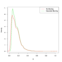
There are errors associated with the modern climate data measurements. Expert opinion 1 suggests that GDD5 measurements may be taken as plus or minus 100 degree days and MTCO as plus or minus 2 degrees. A crude method for correcting for these uncertainties post-hoc is to convolve the cross-validation inverse posterior predictive distributions with a kernel that has a width on this scale.
A 2D truncated Gaussian kernel convolution was applied to each of the leave-one-out posterior predictive distributions for the inverse cross-validation. This has the effect of increasing the variance of the inverse predictive distributions. For example, in the marginals by-taxon model below, convolution with a Gaussian kernel of variance 3 and truncation distance equal to 3 grid spacings was used.
The resulting predictive distributions are still defined on the regular grid. The value at each gridpoint becomes a weighted average of its neighbours, with weights determined by the Gaussian kernel. The truncation of this kernel is for computational reasons; beyond 3 grid spacings the weights are extremely low (0.248% of the central weight) and therefore not computed.
This Gaussian blurring causes the Δ statistic to drop from 34.54% (very poor fit) to 14.2%. This is around half of the non-blurred version. In fact, the slope of the line in Figure 6.6 roughly halves. At the same time, the predictive power statistic D increases from 0.14 to 0.148, representing a loss in accuracy of just 5%. However, this is a crude and somewhat ad-hoc method to account for the uncertainty in the reported climates, the form of which is unknown.
|
|
The results presented above include an explicit modelling of the zero-inflation of the data, as per Section 6.3. If the data is not modelled with a zero-inflated likelihood and an overdispersed likelihood is used, as per Haslett et al. (2006), then the results will differ.
Analysis of the impact of explicit modelling of the extra zeroes was performed through comparison with a model in the spirit of Haslett et al. (2006). Specifically, two models with identical priors for the latent surfaces but with differing likelihoods were fitted to a subset of the data (500 points).
The likelihood for the non zero-inflated model is an overdispersed scaled Poisson for each of the individual taxa. Mixing the Poisson with a Gamma function leads to a negative-Binomial likelihood. Thus, for taxon i at climate location index j
 | (6.10) |
with λij � exij
The zero-inflated model uses a mixture of this likelihood with a point mass at zero. The size of the point mass at zero is 1 � qij
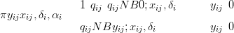 | (6.11) |
with qij � αi
αi
and NByij;xij,δi� given by Equation (6.10).
Thus, for each of the 28 taxa, there are 2 hyperparameters (κi and δi) to be estimated for the first model and 3 hyperparameters (κi, δi and αi) for the zero-inflated model. This zero-inflated negative-Binomial likelihood is the same used to produce the results in this section thus far. Comparison between the results for the two models using the Δ and D inverse cross-validation summary statistics is shown in Table 6.4.4. Also shown is the mean posterior modal value for the overdispersion hyperparameter δi across all taxa i � 1,…,28. These results indicate that the zero-inflated model is a better fit to the data and that the likelihood variance (controlled by δ) is reduced. This leads to higher predictive power, as revealed by a lower mean expected squared distance to the observations D.
|
Section 3.5.6 introduced the concept of nesting structures within compositional counts data. It is demonstrated in that section that lack of appropriate modelling of the nesting will lead to erroneous inferences and that this may manifest as an increased inverse predictive density error as measured by the statistic of the percentage of points lying outside their corresponding 95% highest predicitve density region.
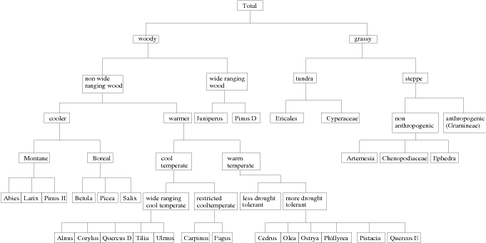
Applying the nesting structure depicted in Figure 6.9 leads to markedly different cross-validation results for the RS10 pollen dataset. This is referred to as the nested model . Although it is disjoint-decomposable, the taxa are no longer modelled as conditionally independent given the climate; the individual components of a nest still are.
Given the nesting structure, errors associated with the inference-via-marginals models are minimized; this is because down to all but the final level in each nest there are only two categories as the preceding nest is divided in a binary split. Thus each nest may be modelled as with Binomial type likelihood and is thus univariate.
The sum-to-unity constraint forces the two components of the split to be perfectly negatively correlated. Any other form of interaction is swamped and cannot therefore impact the model. As only one branch of each split need be modelled (the response of the other is exactly 1 minus the first), normalisation is not required.
For the 28 taxa there are 32 components of the nested model. The overall Δ statistic improved from 14.2% for the by-taxon model to 6.12% for the nested model. Based on this cross-validation statistic, the nested model makes considerably fewer errors for the inverse problem on this dataset.
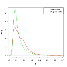
Fortunately, the reduction in error does not appear to come with a reduction of predictive accuracy. The sample density of the D values for the by-taxon marginals model and the nested model is shown in Figure 6.10. The nested model produces lower values for the expected squared distance to the observation, showing greater predictive power in the inverse problem. The mean values for D were found to be
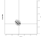
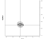
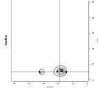
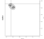
Figure 6.12 shows three example leave-one-out inverse cross-validation predictive densities and the associated left-out points for both the marginals-by taxon model and the nested model, with nested structure as per Figure 6.9.
|
|
|
|
If the nesting structure given by Figure 6.9 is correct then the components of each nest should be conditionally independent, given the climates and the constraint (where there are only two components they are fully negatively correlated and the question is non-applicable).
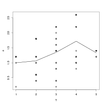
The results of applying the same method of plotting Δ against T as in Section 6.6 for
the nest labeled “more drought tolerant” is shown in Figure 6.11. There is not a wide
range of values across which to evaluate ΔT� (maximum T is 6 taxa) and therefore it is
not straightforward to assess whether Δ varies with T. For all other nests, such
as that labeled “wide ranging cool temperate”, there are even fewer values of
T.
The figure shows that Δ does not increase as more taxa are modelled. This results suggests that the taxa within the “more drought tolerant” nest are conditionally independent, given climate.
|
|
|
The D statistic and the distribution of Dlj� may be used to compare the inverse
predictive power of two or more models. Analysis of the individual expected squared
distances Dlj� is also used to detect outliers as these will have larger than expected D
values, under the fitted model.
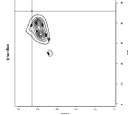
This approach was applied to the pollen training dataset and the highest D value for the nested model was found to be D � 0.661. Figure 6.13 shows the inverse predictive distributions for this datum given the nested model. Examination of the data at that location revealed there to be only two taxa present, Artemesia (sagebrush and wormwood) and Chenopodiaceae , both of which are non-anthropogenic grasses. The reported climate is GDD5� 128 and MTCO ��168, a cold-in-winter climate with a very short growing season. The fitted responses for these taxa show that these grasses thrive in temperate climates. However they are indigenous to the physical region and are hardy. Although they may in fact grow sparsely at that location, they will nevertheless dominate the assemblage. Most interestingly, this outlier is the sampling location with the highest altitude; 5100 metres above sea level, in the mountains in Kashmir.
|
|
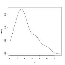
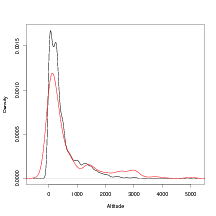
Investigation of the effect of extreme altitude on outliers expands on this result. Defining those data that have a D metric greater than the 95% quantile for D (i.e. the top 5% least well predicted data) to be outliers and plotting the sample density of the altitudes associated with those outlying data reveals thicker tails than the sample density of the entire dataset. This is shown in Figure 6.14.
|
|
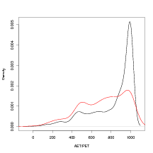
A similar analysis for another climate variable for which data are available is shown in Figure 6.15. In this example, the ratio of actual to potential evapotranspiration (AET/PET) is used. This figure suggests that low values of AET/PET - indicating arid conditions - tend to be less well predicted by the model as the red line (sample density for AET/PET of the subset of the data with the top 5% worst predicted climates) shows a sample with a lower proportion of high values of AET/PET. This indicates that modelling of these AET/PET values should be carried out.
|
|
Figure 6.14 demonstrates that there is a relationship between the altitude of the sampling location and the probability that the datum will be an outlier in the inverse (climate predictive) sense. There are only 9 datapoints whose cross-validation climate predictive distributions place exactly zero probability mass at the correct location. The 9 altitudes, in metres, associated with these locations are

7 out of 9 of these have altitudes that are above the 98% quantile. This again suggests a strong link between extreme altitude and lack of fit. The final two values suggest that this is not the only factor.
The cross-validation model fit statistic Δ is a simple measure of fit; if the model fits the data, then the theory dictates that Δ should be around 5% or less. Simulated data, for which the model is known, in Chapter 4 shows that values as high as 10% are possbile. Values above this have not been observed for toy problems that are on the same scale as the pollen problem.
This allows for a simple, albeit crude, check of model fit to be made. For example, the disjoint-decomposition by-taxon of the model did not appear to be a good model fit to the data. More importantly, a positive linear relationship between the number of taxa used in the model and the Δ statistic was established empirically. This relationship suggests that the disjoint-decomposition by-taxon is a poor model due to a non-zero dependence between the taxa, given the climate.
Comparison between models is performed using the cross-validation statistic D. Dlj�
is the expected squared distance to the climate observation lj, under the model and given
all other data. The lower this value, the more accurately the trained model can predict
or reconstruct climates, given a counts vector. Thus, models with lower D are
preferred.
Δ and D are used constructively to illustrate the importance of modelling advances made since Haslett et al. (2006) such as zero-inflated counts likelihoods. However, the greatest contribution to modelling the RS10 dataset is the delivery of working methods to compare and validate such models, using the INLA based approximation techniques. MCMC based methods fail to achieve this objective due to the computational burden associated with sampling based methods.
Estimation of the various hyperparameters of the model is also performed quickly using approximation methods. This is difficult in the extreme using MCMC based methodology due to issues of mixing.
The discrete grid on which the data are made to lie facilitates fast inversion of the forward model. Normalisation of the posterior for climate, given count is performed numerically. This further speeds up cross-validation in the inverse sense.
A new nested compositional model is introduced. Assessment of the particular nesting structure reported on here shows a marked improvement in this model over the marginals by-taxon model. Most of the apparent conditional dependence between the various plant taxa has been accounted for via the nesting. This is achieved without incurring large computational overhead or developing additional code.
Work has not yet been carried out to determine what value of D determines a model that may be said to fit the data. One method for performing such a calculation is to use Monte-Carlo methods to simulate data from the fitted model; the D statistic based on the simulated data then represents the D value for a model that fits the data.
Although the nested model defined by the diagram in Figure 6.9 leads to a welcome decrease in both Δ and D, it is not clear from these statistics that the model may be said to fit the pollen data. Further criticism of the nesting structure is certainly required; alternative nesting structures should also be explored. The structure in Figure 6.9 is based on expert opinion, but comes with caveats; it is by no means a final statement of definite nesting structure.
Results for models with additional climate dimensions, for which data is available, have not been presented here. Perhaps the by-taxon decomposition of the model is a satisfactory assumption for a 3D climate. Taxa that are not conditionally independent given 2 climate dimensions may be conditionally independent given 3 or more climate variables.
The post-hoc Gaussian-blurring of the climate predictive distributions is ad-hoc and not thoroughly investigated. It is an attempt to account for the uncertainty in the reported climates for the training data in a cheap and simple way. Further thought is required in this area.
Both Δ and D were used with success to identify problematic data. Sampling locations associated with extreme altitudes were found to have an association with being outliers with respect to the fitted model. However, the definition of outlier is not firmly established here and incorporating the altitudes into the model has not been addressed.