Group Testing with Error Correction
Group testing was introduced by R. Dorfman in 1943 to screen US Army recruits for syphilis. The key insight: rather than testing each blood sample individually, combine samples into pools and test the mixture. A pool is positive if and only if it contains at least one defective sample — the Boolean OR of its contents. In the non-adaptive setting studied here, all pools are fixed in advance and all tests run in a single, parallel round. The assignment of samples to pools is encoded by a matrix $G \in \mathbb{B}_2^{N \times K}$, where $N$ is the number of samples and $K$ the number of tests.
Classical non-adaptive group testing assumes perfectly reliable tests. In practice, assays are imperfect. Inexpensive COVID-19 antigen tests — valued precisely for their low cost and rapid turnaround — exhibited false-positive rates around 2% and false-negative rates exceeding 20%. Such assays are however not fully reliable, and standard pooling theory simply breaks down in this setting. The central question of this work is therefore: can the test matrix itself carry sufficient redundancy to detect and correct faulty test results — much as an error-correcting code corrects transmission errors — while simultaneously identifying which samples are defective?
The algebraic framework that makes this possible is Boolean linear algebra over $\mathbb{B}_2 = \{0,1\}$, where addition satisfies $1 + 1 = 1$ rather than $1 \oplus 1 = 0$. This seemingly small difference has deep structural consequences: there is no additive inverse, no Gaussian elimination, no standard coding theory. The natural replacement is residuation theory: every $\mathbb{B}_2$-linear map $f(x) = xG$ has a canonical residual $g(y) = \overline{\,\overline{y} \cdot G^T}$, which in the noiseless case serves directly as the decider: under $t$-disjunctness, $g(xG) = x$ for every infection pattern $x$ with at most $t$ defectives. The condition $t$-disjunctness is precisely the condition under which $g$ inverts $f$, and also admits the most efficient verification algorithm: $O(M)$ rather than $O(M^2)$. In the noisy case, recovering $x$ from a corrupted observation $z$ requires first locating the nearest codeword $c^*$ to $z$ in $C_t$ — a computationally hard problem in general, solved here by brute force over the precomputed code — and then applying $g(c^*)$ as the decider.
Our most powerful examples of group testing schemes arise from finite geometries: projective spaces, affine spaces, Barbilian spaces, transversal designs, inversive planes, and generalized quadrangles. Their combinatorial regularity — constant block size, constant replication number — translates directly into guaranteed disjunctness and error-correction capacity. The Forbes–Gnilke–Greferath theorem gives exact code parameters for Barbilian spaces; the Greferath–Rößing–Wright theorem and its Corollary bound the disjunctness of any Steiner-system-based scheme. The interactive playground allows direct exploration and simulation of all schemes presented here.
The material is based on joint work with J. V. Dinesen, D. Forbes, O. Gnilke, and C. Rößing. See the references for the full list.
The Boolean Semifield $\mathbb{B}_2$
Consider the lattice $\mathbb{B}_2 := \{0, 1\}$ with order $0 < 1$. Its sup and inf operations give it the structure of a semifield, with addition $+$ (Boolean sum) and multiplication $\cdot$ (Boolean product):
| $+$ | $0$ | $1$ |
| $0$ | $0$ | $1$ |
| $1$ | $1$ | $\mathbf{1}$ |
| $\cdot$ | $0$ | $1$ |
| $0$ | $0$ | $0$ |
| $1$ | $0$ | $1$ |
| $\oplus$ | $0$ | $1$ |
| $0$ | $0$ | $1$ |
| $1$ | $1$ | $\mathbf{0}$ |
The critical difference is highlighted: in $\mathbb{B}_2$ we have $1 + 1 = 1$ (gold), whereas in the Galois field $\mathbb{F}_2$ we have $1 \oplus 1 = 0$ (red). Over $\mathbb{B}_2$, there is no additive inverse, and hence no Gaussian elimination. This necessitates a different algebraic framework — residuation theory.
The order $0 < 1$ on $\mathbb{B}_2$ extends componentwise to $\mathbb{B}_2^n$: for $x, y \in \mathbb{B}_2^n$ we write $x \leq y$ if $x_i \leq y_i$ for all $i$, i.e., every component of $x$ that is $1$ is also $1$ in $y$. This makes $\mathbb{B}_2^n$ a distributive lattice, with join (coordinatewise $+$) and meet (coordinatewise $\cdot$).
Let $(A, \leq)$ and $(B, \preceq)$ be partially ordered sets. A pair of mappings $(f, g)$ with $f: A \to B$ and $g: B \to A$ is called a residuated pair if $$f(a) \preceq b \;\Longleftrightarrow\; a \leq g(b) \quad\text{for all } a \in A,\; b \in B.$$ Here $f$ is called residuated and $g$ is called residual.
The componentwise negation on $\mathbb{B}_2$ is the order-reversing involution $\overline{0} = 1$, $\overline{1} = 0$ (logical complement). Unlike subtraction in $\mathbb{F}_2$, this is not an algebraic inverse for addition — it lies outside the semifield operations but is essential for expressing residuals.
A mapping $f: \mathbb{B}_2^N \to \mathbb{B}_2^K$ is $\mathbb{B}_2$-linear if and only if it is residuated. If $f$ is represented by an $N \times K$ matrix $G$ (i.e., $f(x) = xG$), then its residual $g$ is given by $$g(y) \;=\; \overline{\,\overline{y} \cdot G^T\,},$$ where negation is applied componentwise.
For any residuated mapping $f$ with residual $g$, the inequality $$g(f(x)) \;\geq\; x$$ holds componentwise for all $x \in \mathbb{B}_2^N$. The inequality may be strict: $g \circ f$ is not the identity in general, but it is always an upper bound for $x$.
Noiseless Group Testing
In the noiseless model, each test yields a perfectly reliable result. A binary vector $x \in \mathbb{B}_2^N$ represents the infection pattern ($x_i = 1$ if sample $i$ is defective). The test outcome is $y = xG \in \mathbb{B}_2^K$, computed over $\mathbb{B}_2$.
A central question is: can we recover $x$ from $y$, at least when the number of defectives is bounded? We write $w_H(x)$ for the Hamming weight of $x$ — the number of non-zero coordinates of $x$ — which equals the number of defective samples in the pattern $x$. Two conditions on $f$ capture recoverability, and their distinction is both subtle and important:
A group testing scheme $f: \mathbb{B}_2^N \to \mathbb{B}_2^K$ satisfies ($t$-sep) if $f$ is injective on vectors of weight at most $t$: whenever $x, y \in \mathbb{B}_2^N$ with $w_H(x) \leq t$, $w_H(y) \leq t$, and $f(x) = f(y)$, then $x = y$.
The scheme satisfies the stronger condition ($t$-dis) if: whenever $x, y \in \mathbb{B}_2^N$ with $w_H(x) \leq t$ and $f(x) = f(y)$, then $x = y$. Note that here only $x$ is required to have small weight — $y$ is arbitrary. ($t$-dis) is precisely the condition under which equality $g(f(x)) = x$ holds for all $x$ with $w_H(x) \leq t$: the residual identifies the infection pattern exactly, producing neither false negatives (missed defectives) nor false positives (healthy samples declared defective).
Both conditions are monotone: ($t$-dis) implies ($s$-dis) for all $s \leq t$, and likewise for ($t$-sep). This is immediate from the definitions, since $w_H(x) \leq s$ implies $w_H(x) \leq t$. We therefore speak of the maximum disjunctness of a scheme — the largest $t$ for which ($t$-dis) holds.
The condition ($t$-sep) merely says that different infection patterns of weight $\leq t$ produce different test outcomes — the mapping is invertible in principle. The condition ($t$-dis) is strictly stronger: it guarantees that no vector outside the Hamming ball can collide with one inside it. This has a decisive practical consequence:
The scheme represented by $G$ satisfies ($t$-dis) if and only if the residual mapping $g(y) = \overline{\,\overline{y} \cdot G^T}$ inverts $f$ on all $x \in \mathbb{B}_2^N$ with $w_H(x) \leq t$, i.e., $g(f(x)) = x$.
In other words: ($t$-dis) is equivalent to the statement that the residual mapping $g$ itself serves as an efficient, constructive decider — it directly recovers the infection pattern without any further search. Under ($t$-sep) alone, a unique solution exists in principle, but the residual is not guaranteed to find it.
Remarkably, the stronger property admits a more efficient verification. The interactive tool below uses this residuation-based approach.
A Small Example: a Binary Test Matrix
The $10 \times 6$ matrix $G$ below assigns 10 samples (1–10) to 6 test pools (A–F). Entry $G_{ij} = 1$ means sample $i$ participates in pool $j$.
| A | B | C | D | E | F | |
| 1 | 1 | 1 | 0 | 1 | 0 | 0 |
| 2 | 1 | 0 | 1 | 0 | 1 | 0 |
| 3 | 1 | 0 | 0 | 0 | 0 | 1 |
| 4 | 0 | 1 | 1 | 0 | 0 | 1 |
| 5 | 0 | 1 | 0 | 0 | 1 | 1 |
| 6 | 0 | 0 | 1 | 1 | 0 | 1 |
| 7 | 0 | 0 | 0 | 1 | 1 | 0 |
| 8 | 1 | 0 | 0 | 0 | 1 | 1 |
| 9 | 0 | 1 | 1 | 0 | 1 | 0 |
| 10 | 0 | 0 | 1 | 1 | 0 | 0 |
If samples 3 and 7 are defective, the infection pattern is $x = (0,0,1,0,0,0,1,0,0,0)$ and the test outcome is $$y \;=\; xG \;=\; (1,0,0,1,1,1) \;\in\; \mathbb{B}_2^6{:}$$ pools A, D, E, F positive; pools B, C negative.
Since $1 + 1 = 1$ in $\mathbb{B}_2$, a pool tests positive as soon as at least one of its samples is defective — the algebraic expression of the key property of group testing.
Noisy Group Testing
In practice, tests may be unreliable. Experience with antigen tests during the COVID-19 pandemic shows that false-positive rates around 2% and false-negative rates exceeding 20% are realistic. We model test errors using the Hamming distance on $\mathbb{B}_2^K$. This is admittedly a simplification: the Hamming metric treats false positives and false negatives as equally costly, whereas in reality they arise with markedly different probabilities. A non-symmetric distance function — analogous to the Z-channel metric familiar from information theory — would be the more faithful model. Whether and how such an asymmetric metric can be integrated into the residuation-based framework is a natural question for further investigation.
Remark. Lack of reliability is often associated with inexpensive tests: a less expensive assay tends to be less accurate. Error-correcting group testing offers a practical trade-off — it can compensate for reduced reliability without requiring one to pay for more expensive, higher-accuracy tests.
In classical noiseless group testing, the primary goal is to minimise the number of tests $K$ relative to the number of participants $N$. This remains a valid and important objective. However, when tests are unreliable, the scheme must carry redundancy to enable error detection or correction — and redundancy requires additional tests. Depending on the error probability and the desired correction capability, this may lead to $K$ close to $N$, equal to $N$, or even $K > N$.
Caveat: Over $\mathbb{B}_2$, the Hamming distance does not enjoy all its familiar properties — in particular, it is not translation-invariant, since $\mathbb{B}_2$ has no subtraction. At least the following expression remains valid: $$d_H(x, y) \;=\; w_H(x) + w_H(y) - 2\,w_H(x \cdot y),$$ where $x \cdot y$ denotes the coordinatewise (Schur/Hadamard) product.
Codes over $\mathbb{B}_2$
Given a test matrix $G \in \mathbb{B}_2^{N \times K}$, used here as the generator matrix of a Boolean code, and a non-negative integer $s$, we define the code $$C_s \;=\; B_N(s, 0) \cdot G \;=\; \{x G \mid x \in \mathbb{B}_2^N,\; w_H(x) \leq s\},$$ where $B_N(s, 0)$ is the Hamming ball of radius $s$ around the origin. The minimum distance $d_\min(C_s)$ determines the error-correction capability: up to $e = \lfloor(d_\min - 1)/2\rfloor$ faulty test results can be corrected.
As $s$ ranges from $0$ to $N$, these codes form a nested chain: $$\{0\} \;=\; C_0 \;\subseteq\; C_1 \;\subseteq\; \cdots \;\subseteq\; C_N \;=\; \langle G \rangle,$$ where $\langle G \rangle \subseteq \mathbb{B}_2^K$ denotes the row space of $G$, with minimum distances decreasing along the chain — identifying more defectives leaves less room for error correction. In practice we stop at $s = t$, the target disjunctness level, since larger $s$ adds codewords that cannot be decoded by residuation.
Incidence Structures and Designs
The most effective group testing matrices do not arise by chance — they are incidence matrices of finite geometries, combinatorial structures whose regularity translates directly into disjunctness and error-correction guarantees.
An incidence structure is a triple $(P, \mathcal{B}, I)$ where $P$ is a finite set of $v$ points, $\mathcal{B}$ is a finite set of $b$ blocks, and $I \subseteq P \times \mathcal{B}$ is the incidence relation. A matrix $M \in \mathbb{B}_2^{b \times v}$ is called an incidence matrix for $(P, \mathcal{B}, I)$ if $M_{Bp} = 1$ whenever $(p, B) \in I$, and $M_{Bp} = 0$ otherwise.
An incidence matrix is determined by $(P, \mathcal{B}, I)$ only up to permutations of its rows and columns (relabellings of blocks and points); it is therefore not unique in the strict sense. The dual of $(P, \mathcal{B}, I)$ is the incidence structure $(\mathcal{B}, P, I^*)$ with $I^* = \{(B, p) : (p, B) \in I\}$; its incidence matrix is $M^T$.
For group testing we identify blocks with samples ($N = b$) and points with tests ($K = v$), so any incidence matrix $M$ serves directly as the test matrix $G = M \in \mathbb{B}_2^{N \times K}$. Passing to the dual yields $G = M^T$, giving a GT scheme on the same geometry with points as samples and blocks as tests. Both orientations may be used in practice.
A $t$-$(v, k, \lambda)$ design is an incidence structure $(P, \mathcal{B}, I)$ in which every block has the same size $k$, and every $t$-element subset of points is contained in exactly $\lambda$ blocks. The total block count is $$b \;=\; \lambda\,\binom{v}{t}\Big/\binom{k}{t}.$$ The regularity of a design constrains the row and column sums of the test matrix, which in turn controls the disjunctness and code distances of the associated group testing scheme.
Let $(P, \mathcal{B}, I)$ be a $t$-$(v, k, 1)$ design (Steiner system), and let $B_1, \ldots, B_m$ be a collection of $m$ distinct blocks. Suppose $k > (t-1)m$. Then:
- $\left|B_1 \cup \cdots \cup B_m\right| \;\geq\; mk \;-\; (t-1)\,\dfrac{m(m-1)}{2}.$
- If a block $B \in \mathcal{B}$ satisfies $B \subseteq B_1 \cup \cdots \cup B_m$, then $B = B_j$ for some $1 \leq j \leq m$; in particular, $B$ is uniquely determined.
Let $(P, \mathcal{B}, I)$ be a $t$-$(v, k, 1)$ design (Steiner system) used as a GT scheme with blocks as samples ($N = b$), points as tests ($K = v$), and test matrix $G = M \in \mathbb{B}_2^{N \times K}$. Then $k$ is the row weight of $G$ — the number of points per block, which equals the number of tests per sample. The scheme is $s$-disjunct for every positive integer $s$ satisfying $s < k/(t-1)$. In particular, it is $$\left\lfloor \frac{k-1}{t-1} \right\rfloor\text{-disjunct.}$$
Proof. Let $G_i \in \mathbb{B}_2^K$ denote the $i$-th row of $G$ (the characteristic vector of block $i$). From the residual formula $g(y) = \overline{\,\overline{y} \cdot G^T\,}$ one reads off directly: $$g(y)_i = 1 \;\iff\; G_i \leq y.$$ Now let $x \in \mathbb{B}_2^N$ with $w_H(x) = m \leq s$, and set $y = xG$.
Case $x_i = 1$. Then $y_j \geq x_i G_{ij} = G_{ij}$ for all $j$, so $G_i \leq y$, hence $g(y)_i = 1$. (This is the Observation of Section 1, applied componentwise.)
Case $x_i = 0$. Suppose for contradiction that $G_i \leq y$. Let $B_1, \ldots, B_m$ be the blocks indexed by $\mathrm{supp}(x)$. Since $y = xG$, the condition $G_i \leq y$ means precisely that $B_i \subseteq B_1 \cup \cdots \cup B_m$. The hypothesis $s < k/(t-1)$ gives $k > (t-1)m$, so part (b) of the theorem forces $B_i = B_\ell$ for some $\ell$, contradicting $x_i = 0$. Hence $G_i \not\leq y$, so $g(y)_i = 0$.
Together: $g(y)_i = 1 \iff x_i = 1$ for all $i$, i.e.\ $g(y) = x$. □
Projective Geometry $\mathrm{PG}(d,q)$
For a prime power $q$, let $\mathbb{F}_q$ be the finite field of order $q$. The projective space $\mathrm{PG}(d, q)$ is the incidence structure $(P, \mathcal{B}, I)$, where $P$ is the set of all 1-dimensional subspaces (points), $\mathcal{B}$ is the set of all 2-dimensional subspaces (lines) of $\mathbb{F}_q^{d+1}$, and $I = \{\,(p, L) : p \subseteq L\,\}$ is subspace containment. The point count and line count are, respectively, $$v \;=\; \frac{q^{d+1}-1}{q-1}, \qquad b \;=\; \frac{(q^{d+1}-1)(q^d-1)}{(q-1)(q^2-1)}.$$ Each line contains exactly $q+1$ points, and any two distinct points determine a unique line, making $(P, \mathcal{B}, I)$ a $2$-$\!\left(v,\; q+1,\; 1\right)$ Steiner system. Two natural families of subspaces serve as blocks for GT schemes.
The Fano Plane $\mathrm{PG}(2,2)$
The smallest projective space that is not a single line is known as the Fano plane $\mathrm{PG}(2,2)$. It contains $v = 7$ points and $b = 7$ lines, each line passing through exactly $3$ points and each point lying on exactly $3$ lines. It hence forms a $2$-$(7,3,1)$ Steiner system $(P, \mathcal{B}, I)$; as $d=2$, this structure is self-dual, and therefore both GT orientations yield the same $7 \times 7$ matrix. The Corollary gives $2$-disjunctness, confirmed in the playground.
| Scheme | Design | $N \times K$ | max disjunctness | $d_{\min}(C_1)$ | $d_{\min}(C_2)$ |
|---|---|---|---|---|---|
| $\mathrm{PG}(2,2)$ / Fano | $2$-$(7,3,1)$ | $7 \times 7$ | $2$ | $3$ | $2$ |
Lines as samples for GT
With lines as samples ($N = b$) and points as tests ($K = v$), the Corollary applies with $t = 2$ and $k = q+1$:
For any $d \geq 2$ and prime power $q$, the GT scheme obtained from $\mathrm{PG}(d,q)$ by taking lines as samples and points as tests is $q$-disjunct.
Hyperplanes as samples for GT
The hyperplanes of $\mathrm{PG}(d,q)$ are the $(d-1)$-dimensional projective subspaces; there are again $$v \;=\; \frac{q^{d+1}-1}{q-1}$$ of them, so the incidence matrix $M$ is square ($N = K = v$). Any two points lie together in $\lambda = \frac{q^{d-1}-1}{q-1}$ hyperplanes, making this a $2$-design that is not a Steiner system in general, so that the Corollary does not directly apply. This family is studied in depth as Barbilian spaces in the next section.
Group Testing with Barbilian Spaces
Let $\mathbb{F}_q$ be a finite field and $d \geq 2$. The Barbilian space $\mathrm{Barb}(d, q)$ is the incidence structure $(P, \mathcal{H}, I)$ of $\mathrm{PG}(d, q)$, where $P$ is the set of points, $\mathcal{H}$ is the set of hyperplanes ($(d-1)$-dimensional subspaces), and $I = \{(p, h) : p \in h\}$. With hyperplanes as samples ($N = |\mathcal{H}|$) and points as tests ($K = |P|$), and noting $|\mathcal{H}| = |P| = \frac{q^{d+1}-1}{q-1}$, the scheme is square ($N = K$) and forms a $2$-$\big(\frac{q^{d+1}-1}{q-1},\; \frac{q^d-1}{q-1},\; \frac{q^{d-1}-1}{q-1}\big)$ design.
For a prime power $q$ and integer $d \geq 2$, let $G$ be an incidence matrix of $\mathrm{Barb}(d, q)$. Then:
- The scheme tests $N = \frac{q^{d+1}-1}{q-1}$ participants using $K = N$ tests.
- Its maximum disjunctness is $t = q$.
- The minimum distance of $C_t = B_N(t, 0) \cdot G$ is: $$d_\min \;=\; \begin{cases} \dfrac{q^d - 1}{q-1} & \text{if } t = 1,\\[6pt] q^{d-1} - (t-2)\,q^{d-2} & \text{if } 2 \leq t \leq q.\end{cases}$$
Remark (Prior work). The bound $t = q$ for $d \geq 3$ was obtained independently by D'yachkov, Hwang, Macula, Vilenkin, and Weng [7] as a special case of their Corollary 4.8, via the containment matrix $M(d{+}1,\, d,\, 1)$ of points and hyperplanes in $\mathrm{PG}(d, q)$. Their argument requires $d \geq 3$ and does not address the case $d = 2$, nor the minimum distances of $C_t$ at each level.
The Barbilian spaces happen to produce schemes with $K = N$, a consequence of the inner symmetry of the underlying projective geometry (points and hyperplanes are equinumerous). They are one family of examples — not the final word on the matter. In general, the problem of minimising $K$ subject to a given $t$-disjunctness and a given error-correction guarantee remains wide open.
To appreciate the value of pooling, consider the trivial alternative: the $N \times N$ identity matrix $I_N$ also has $K = N$ and maximum disjunctness $t = N$ — it identifies any number of defectives. Yet its codes $C_t$ have $d_\min = 1$ for every $t \geq 1$: a single faulty test causes misidentification with no possibility of detection. Pooling is the mechanism that converts tests into redundancy and hence into robustness.
Code Properties by Scheme
| Scheme | $t$ | $|C_t|$ | $d_{\min}$ | Error handling |
|---|---|---|---|---|
| $\mathrm{Barb}(2,2)$ $N = K = 7$ |
$1$ | 8 | $3$ | corrects 1 error |
| $2$ | 29 | $2$ | detects 1 error | |
| $\mathrm{Barb}(3,2)$ $N = K = 15$ |
$1$ | 16 | $7$ | corrects 3 errors |
| $2$ | 121 | $4$ | corrects 1 error | |
| $\mathrm{Barb}(4,2)$ $N = K = 31$ |
$1$ | 32 | $15$ | corrects 7 errors |
| $2$ | 497 | $8$ | corrects 3 errors | |
| $\mathrm{Barb}(2,5)$ $N = K = 31$ |
$1$ | 32 | $6$ | corrects 2 errors |
| $2$ | 497 | $5$ | corrects 2 errors | |
| $3$ | 4,992 | $4$ | corrects 1 error | |
| $4$ | 36,457 | $3$ | corrects 1 error | |
| $5$ | 206,368 | $2$ | detects 1 error |
Highlighted rows: maximum disjunctness level. Values for $\mathrm{Barb}(2,2)$–$\mathrm{Barb}(4,2)$ confirmed by both the Forbes–Gnilke–Greferath theorem and direct computation. Values for $\mathrm{Barb}(2,5)$ from direct computation (corrected from earlier FGG estimates).
Affine Geometry $\mathrm{AG}(d,q)$
The affine space $\mathrm{AG}(d,q)$ is obtained from $\mathrm{PG}(d,q)$ by removing a fixed hyperplane (the hyperplane at infinity) together with all its subspaces. It has $v = q^d$ affine points. The remaining subspaces, called $r$-flats for $r = 1, \ldots, d{-}1$, form natural families of blocks; incidence is again subspace containment. For each choice of $r$, the incidence structure $(P, \mathcal{B}_r, I_r)$ of affine points and $r$-flats yields a GT scheme with $r$-flats as samples and points as tests.
The affine plane $\mathrm{AG}(2, q)$ has $v = q^2$ points and $b = q^2 + q$ lines, partitioned into $q+1$ parallel classes of $q$ lines each. Any two points determine a unique line, making the line incidence structure a $2$-$(q^2, q, 1)$ Steiner system. With lines as samples ($N = q^2+q$) and points as tests ($K = q^2$), the Corollary applies with $t = 2$ and $k = q$:
For any prime power $q$, the GT scheme obtained from $\mathrm{AG}(2,q)$ by taking lines as samples and points as tests is $(q-1)$-disjunct.
For $d \geq 3$, the $r$-flats of $\mathrm{AG}(d,q)$ for $r \in \{1, d{-}1\}$ provide further GT schemes. The table below lists all affine playground presets; exact disjunctness and $d_{\min}$ values are listed in the table below.
| Scheme | Blocks | $t$ | $|C_t|$ | $d_{\min}$ | Error handling |
|---|---|---|---|---|---|
| $\mathrm{AG(2,4)}$ $N\!\times\!K=20\times 16$ |
lines, $2$-$(16,4,1)$ | $1$ | 21 | $4$ | corrects 1 error |
| $2$ | 211 | $3$ | corrects 1 error | ||
| $3$ | 1,351 | $2$ | detects 1 error | ||
| $\mathrm{AG(2,5)}$ $N\!\times\!K=30\times 25$ |
lines, $2$-$(25,5,1)$ | $1$ | 31 | $5$ | corrects 2 errors |
| $2$ | 466 | $4$ | corrects 1 error | ||
| $3$ | 4,526 | $3$ | corrects 1 error | ||
| $4$ | 31,931 | $2$ | detects 1 error | ||
| $\mathrm{AG(2,7)}$ $N\!\times\!K=56\times 49$ |
lines, $2$-$(49,7,1)$ | $1$ | 57 | $7$ | corrects 3 errors |
| $2$ | 1,597 | $6$ | corrects 2 errors | ||
| $3$ | 29,317 | $5$ | corrects 2 errors | ||
| $4$ | 396,607 | $4$ | corrects 1 error | ||
| $5$ | 4,216,423 | $3$ | corrects 1 error | ||
| $6$ | 36,684,859 | $2$ | detects 1 error | ||
| $\mathrm{AG(3,2)}$ $N\!\times\!K=28\times 8$ |
lines | $1$ | 29 | $2$ | detects 1 error |
| hyperplanes | $1$ | 15 | $4$ | corrects 1 error | |
| $\mathrm{AG(3,3)}$ $N\!\times\!K=117\times 27$ |
lines | $1$ | 118 | $3$ | corrects 1 error |
| $2$ | 6,904 | $2$ | detects 1 error | ||
| hyperplanes | $1$ | 40 | $9$ | corrects 4 errors | |
| $2$ | 781 | $6$ | corrects 2 errors | ||
| $\mathrm{AG(3,4)}$ $N\!\times\!K=84\times 64$ |
hyperplanes | $1$ | 85 | $16$ | corrects 7 errors |
| $2$ | 3,571 | $12$ | corrects 5 errors | ||
| $3$ | 98,855 | $8$ | corrects 3 errors | ||
| $\mathrm{AG(4,2)}$ $N\!\times\!K=120/140/30\times 16$ |
lines | $1$ | 121 | $2$ | detects 1 error |
| $2$-flats | $1$ | 141 | $4$ | corrects 1 error | |
| hyperplanes | $1$ | 31 | $8$ | corrects 3 errors |
Highlighted rows: maximum disjunctness. All $t_{\max}$ values confirm the Corollary ($t_{\max} = q-1$ for $\mathrm{AG}(2,q)$ lines).
Transversal Designs $\mathrm{TD}(k, n)$
A transversal design $\mathrm{TD}(k, n)$ is an incidence structure $(P, \mathcal{B}, I)$ with $|P| = kn$ points partitioned into $k$ groups of $n$ and $|\mathcal{B}| = n^2$ blocks, such that every block contains exactly one point from each group, and any two points from different groups appear together in exactly one block. It forms a $1$-$(kn,\, k,\, 1)$ design.
With blocks as samples ($N = n^2$) and points as tests ($K = kn$), the test matrix is $G = M \in \mathbb{B}_2^{n^2 \times kn}$. Since $\mathrm{TD}(k,n)$ is a $1$-design (not a Steiner system for $t\geq 2$), the Corollary does not directly apply; disjunctness is determined computationally.
Existence. $\mathrm{TD}(k, n)$ exists if and only if there are $k-2$ mutually orthogonal Latin squares (MOLS) of order $n$. In particular, whenever $n = p^r$ is a prime power and $k \leq n + 1$, a $\mathrm{TD}(k,n)$ can be constructed from the affine plane $\mathrm{AG}(2, n)$ by selecting $k$ of its $n+1$ parallel classes.
| Scheme | $t$ | $|C_t|$ | $d_{\min}$ | Error handling |
|---|---|---|---|---|
| $\mathrm{TD(3,5)}$ $N\!\times\!K=25\times 15$ |
$1$ | 26 | $3$ | corrects 1 error |
| $2$ | 326 | $2$ | detects 1 error | |
| $\mathrm{TD(4,5)}$ $N\!\times\!K=25\times 20$ |
$1$ | 26 | $4$ | corrects 1 error |
| $2$ | 326 | $3$ | corrects 1 error | |
| $3$ | 2,626 | $2$ | detects 1 error | |
| $\mathrm{TD(5,5)}$ $N\!\times\!K=25\times 25$ |
$1$ | 26 | $5$ | corrects 2 errors |
| $2$ | 326 | $4$ | corrects 1 error | |
| $3$ | 2,626 | $3$ | corrects 1 error | |
| $4$ | 15,276 | $2$ | detects 1 error | |
| $\mathrm{TD(3,7)}$ $N\!\times\!K=49\times 21$ |
$1$ | 50 | $3$ | corrects 1 error |
| $2$ | 1,226 | $2$ | detects 1 error | |
| $\mathrm{TD(3,7)}^\dagger$ $N\!\times\!K=21\times 49$ |
$1$ | 22 | $7$ | corrects 3 errors |
| $2$ | 232 | $6$ | corrects 2 errors | |
| $3$ | 1,562 | $5$ | corrects 2 errors | |
| $4$ | 7,547 | $4$ | corrects 1 error | |
| $5$ | 27,896 | $3$ | corrects 1 error | |
| $6$ | 82,160 | $2$ | detects 1 error | |
| $\mathrm{TD(4,7)}$ $N\!\times\!K=49\times 28$ |
$1$ | 50 | $4$ | corrects 1 error |
| $2$ | 1,226 | $3$ | corrects 1 error | |
| $3$ | 19,650 | $2$ | detects 1 error | |
| $\mathrm{TD(4,7)}^\dagger$ $N\!\times\!K=28\times 49$ |
$1$ | 29 | $7$ | corrects 3 errors |
| $2$ | 407 | $6$ | corrects 2 errors | |
| $3$ | 3,683 | $5$ | corrects 2 errors | |
| $4$ | 24,158 | $4$ | corrects 1 error | |
| $5$ | 122,438 | $3$ | corrects 1 error | |
| $6$ | 499,178 | $2$ | detects 1 error | |
| $\mathrm{TD(5,7)}$ $N\!\times\!K=49\times 35$ |
$1$ | 50 | $5$ | corrects 2 errors |
| $2$ | 1,226 | $4$ | corrects 1 error | |
| $3$ | 19,650 | $3$ | corrects 1 error | |
| $4$ | 231,526 | $2$ | detects 1 error | |
| $\mathrm{TD(5,7)}^\dagger$ $N\!\times\!K=35\times 49$ |
$1$ | 36 | $7$ | corrects 3 errors |
| $2$ | 631 | $6$ | corrects 2 errors | |
| $3$ | 7,176 | $5$ | corrects 2 errors | |
| $4$ | 59,536 | $4$ | corrects 1 error | |
| $5$ | 384,168 | $3$ | corrects 1 error | |
| $6$ | 2,007,328 | $2$ | detects 1 error | |
| $\mathrm{TD(6,7)}$ $N\!\times\!K=49\times 42$ |
$1$ | 50 | $6$ | corrects 2 errors |
| $2$ | 1,226 | $5$ | corrects 2 errors | |
| $3$ | 19,650 | $4$ | corrects 1 error | |
| $4$ | 231,526 | $3$ | corrects 1 error | |
| $5$ | 2,138,410 | $2$ | detects 1 error | |
| $\mathrm{TD(6,7)}^\dagger$ $N\!\times\!K=42\times 49$ |
$1$ | 43 | $7$ | corrects 3 errors |
| $2$ | 904 | $6$ | corrects 2 errors | |
| $3$ | 12,384 | $5$ | corrects 2 errors | |
| $4$ | 124,314 | $4$ | corrects 1 error | |
| $5$ | 974,982 | $3$ | corrects 1 error | |
| $6$ | 6,220,768 | $2$ | detects 1 error | |
| $\mathrm{TD(7,7)}$ $N\!\times\!K=49\times 49$ |
$1$ | 50 | $7$ | corrects 3 errors |
| $2$ | 1,226 | $6$ | corrects 2 errors | |
| $3$ | 19,650 | $5$ | corrects 2 errors | |
| $4$ | 231,526 | $4$ | corrects 1 error | |
| $5$ | 2,138,410 | $3$ | corrects 1 error | |
| $6$ | 16,122,226 | $2$ | detects 1 error | |
| $\mathrm{TD(8,7)}$ $N\!\times\!K=49\times 56$ |
$1$ | 50 | $8$ | corrects 3 errors |
| $2$ | 1,226 | $7$ | corrects 3 errors | |
| $3$ | 19,650 | $6$ | corrects 2 errors | |
| $4$ | 231,526 | $5$ | corrects 2 errors | |
| $5$ | 2,138,410 | $4$ | corrects 1 error | |
| $6$ | 16,122,226 | $3$ | corrects 1 error | |
| $7$ | 102,022,810 | $2$ | detects 1 error | |
| $\mathrm{TD(8,7)}^\dagger$ $N\!\times\!K=56\times 49$ |
$1$ | 57 | $7$ | corrects 3 errors |
| $2$ | 1,597 | $6$ | corrects 2 errors | |
| $3$ | 29,317 | $5$ | corrects 2 errors | |
| $4$ | 396,607 | $4$ | corrects 1 error | |
| $5$ | 4,216,423 | $3$ | corrects 1 error | |
| $6$ | 36,684,859 | $2$ | detects 1 error | |
| $\mathrm{TD(3,11)}$ $N\!\times\!K=121\times 33$ |
$1$ | 122 | $3$ | corrects 1 error |
| $2$ | 7,382 | $2$ | detects 1 error | |
| $\mathrm{TD(3,11)}^\dagger$ $N\!\times\!K=33\times 121$ |
$1$ | 34 | $11$ | corrects 5 errors |
| $2$ | 562 | $10$ | corrects 4 errors | |
| $3$ | 6,018 | $9$ | corrects 4 errors | |
| $4$ | 46,938 | $8$ | corrects 3 errors | |
| $5$ | 284,274 | $7$ | corrects 3 errors | |
| $6$ | 1,391,842 | $6$ | corrects 2 errors | |
| $7$ | 5,663,890 | $5$ | corrects 2 errors | |
| $\mathrm{TD(4,11)}$ $N\!\times\!K=121\times 44$ |
$1$ | 122 | $4$ | corrects 1 error |
| $2$ | 7,382 | $3$ | corrects 1 error | |
| $3$ | 295,362 | $2$ | detects 1 error | |
| $\mathrm{TD(4,11)}^\dagger$ $N\!\times\!K=44\times 121$ |
$1$ | 45 | $11$ | corrects 5 errors |
| $2$ | 991 | $10$ | corrects 4 errors | |
| $3$ | 14,235 | $9$ | corrects 4 errors | |
| $4$ | 149,986 | $8$ | corrects 3 errors | |
| $5$ | 1,235,994 | $7$ | corrects 3 errors | |
| $6$ | 8,295,046 | $6$ | corrects 2 errors | |
| $7$ | 46,615,614 | $5$ | corrects 2 errors | |
| $\mathrm{TD(5,11)}$ $N\!\times\!K=121\times 55$ |
$1$ | 122 | $5$ | corrects 2 errors |
| $2$ | 7,382 | $4$ | corrects 1 error | |
| $3$ | 295,362 | $3$ | corrects 1 error | |
| $4$ | 8,790,772 | $2$ | detects 1 error | |
| $\mathrm{TD(5,11)}^\dagger$ $N\!\times\!K=55\times 121$ |
$1$ | 56 | $11$ | corrects 5 errors |
| $2$ | 1,541 | $10$ | corrects 4 errors | |
| $3$ | 27,776 | $9$ | corrects 4 errors | |
| $4$ | 368,831 | $8$ | corrects 3 errors | |
| $5$ | 3,847,592 | $7$ | corrects 3 errors | |
| $6$ | 32,837,267 | $6$ | corrects 2 errors | |
| $7$ | 235,764,992 | $5$ | corrects 2 errors | |
| $\mathrm{TD(6,11)}$ $N\!\times\!K=121\times 66$ |
$1$ | 122 | $6$ | corrects 2 errors |
| $2$ | 7,382 | $5$ | corrects 2 errors | |
| $3$ | 295,362 | $4$ | corrects 1 error | |
| $4$ | 8,790,772 | $3$ | corrects 1 error | |
| $5$ | 207,583,366 | $2$ | detects 1 error | |
| $\mathrm{TD(7,11)}$ $N\!\times\!K=121\times 77$ |
$1$ | 122 | $7$ | corrects 3 errors |
| $2$ | 7,382 | $6$ | corrects 2 errors | |
| $3$ | 295,362 | $5$ | corrects 2 errors | |
| $4$ | 8,790,772 | $4$ | corrects 1 error | |
| $5$ | 207,583,366 | $3$ | corrects 1 error | |
| $\mathrm{TD(8,11)}$ $N\!\times\!K=121\times 88$ |
$1$ | 122 | $8$ | corrects 3 errors |
| $2$ | 7,382 | $7$ | corrects 3 errors | |
| $3$ | 295,362 | $6$ | corrects 2 errors | |
| $4$ | 8,790,772 | $5$ | corrects 2 errors | |
| $5$ | 207,583,366 | $4$ | corrects 1 error | |
| $\mathrm{TD(9,11)}$ $N\!\times\!K=121\times 99$ |
$1$ | 122 | $9$ | corrects 4 errors |
| $2$ | 7,382 | $8$ | corrects 3 errors | |
| $3$ | 295,362 | $7$ | corrects 3 errors | |
| $4$ | 8,790,772 | $6$ | corrects 2 errors | |
| $5$ | 207,583,366 | $5$ | corrects 2 errors | |
| $\mathrm{TD(11,11)}$ $N\!\times\!K=121\times 121$ |
$1$ | 122 | $11$ | corrects 5 errors |
| $2$ | 7,382 | $10$ | corrects 4 errors | |
| $3$ | 295,362 | $9$ | corrects 4 errors | |
| $4$ | 8,790,772 | $8$ | corrects 3 errors | |
| $5$ | 207,583,366 | $7$ | corrects 3 errors | |
| $\mathrm{TD(12,11)}$ $N\!\times\!K=121\times 132$ |
$1$ | 122 | $12$ | corrects 5 errors |
| $2$ | 7,382 | $11$ | corrects 5 errors | |
| $3$ | 295,362 | $10$ | corrects 4 errors | |
| $4$ | 8,790,772 | $9$ | corrects 4 errors | |
| $5$ | 207,583,366 | $8$ | corrects 3 errors | |
| $\mathrm{TD(3,13)}$ $N\!\times\!K=169\times 39$ |
$1$ | 170 | $3$ | corrects 1 error |
| $2$ | 14,366 | $2$ | detects 1 error | |
| $\mathrm{TD(3,13)}^\dagger$ $N\!\times\!K=39\times 169$ |
$1$ | 40 | $13$ | corrects 6 errors |
| $2$ | 781 | $12$ | corrects 5 errors | |
| $3$ | 9,920 | $11$ | corrects 5 errors | |
| $4$ | 92,171 | $10$ | corrects 4 errors | |
| $5$ | 667,928 | $9$ | corrects 4 errors | |
| $6$ | 3,930,551 | $8$ | corrects 3 errors | |
| $7$ | 19,311,488 | $7$ | corrects 3 errors | |
| $\mathrm{TD(4,13)}$ $N\!\times\!K=169\times 52$ |
$1$ | 170 | $4$ | corrects 1 error |
| $2$ | 14,366 | $3$ | corrects 1 error | |
| $3$ | 804,610 | $2$ | detects 1 error | |
| $\mathrm{TD(4,13)}^\dagger$ $N\!\times\!K=52\times 169$ |
$1$ | 53 | $13$ | corrects 6 errors |
| $2$ | 1,379 | $12$ | corrects 5 errors | |
| $3$ | 23,479 | $11$ | corrects 5 errors | |
| $4$ | 294,204 | $10$ | corrects 4 errors | |
| $5$ | 2,893,164 | $9$ | corrects 4 errors | |
| $6$ | 23,251,684 | $8$ | corrects 3 errors | |
| $7$ | 157,036,244 | $7$ | corrects 3 errors | |
| $\mathrm{TD(5,13)}$ $N\!\times\!K=169\times 65$ |
$1$ | 170 | $5$ | corrects 2 errors |
| $2$ | 14,366 | $4$ | corrects 1 error | |
| $3$ | 804,610 | $3$ | corrects 1 error | |
| $4$ | 33,599,736 | $2$ | detects 1 error |
Highlighted rows: maximum disjunctness.
Circle Geometries
The three classical Benz circle geometries — inversive (Möbius) planes, Laguerre planes, and Minkowski planes — arise as incidence structures associated with the three types of quadratic ring extensions of $\mathrm{GF}(q)$: the field extension $\mathrm{GF}(q^2)$, the dual-number ring $\mathrm{GF}(q)[\varepsilon]$, and the split extension $\mathrm{GF}(q)\times\mathrm{GF}(q)$, respectively. Each geometry yields a family of highly structured group-testing schemes whose properties are investigated below.
Inversive Planes (Möbius Planes) $\mathbb{M}_q$
An inversive plane of order $q$ is an incidence structure $(P, \mathcal{B}, I)$ with $|P| = q^2+1$ points and $|\mathcal{B}| = q(q^2+1)$ blocks called circles, each circle containing $q+1$ points, such that any three points determine a unique circle. It forms a $3$-$(q^2+1,\, q+1,\, 1)$ Steiner system. With circles as samples ($N = q(q^2+1)$) and points as tests ($K = q^2+1$), the Corollary applies with $t = 3$ and $k = q+1$:
For any prime power $q$, the GT scheme obtained from an inversive plane of order $q$ by taking circles as samples and points as tests is $\left\lfloor q/2 \right\rfloor$-disjunct.
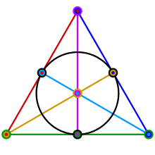
The Möbius Plane $\mathbb{M}_2$
The smallest inversive plane is $\mathbb{M}_2$ of order $q = 2$: a $3$-$(5, 3, 1)$ design with 5 points and 10 circles. Its incidence matrix provides a $(10, 5)$-group testing scheme with maximum disjunctness $t = 1$, identifying a single defective among 10 samples using only 5 tests.

Drawing by Cornelia Rößing †
| A | B | C | D | E | |
| 1 | 1 | 0 | 1 | 0 | 1 |
| 2 | 0 | 1 | 1 | 1 | 0 |
| 3 | 1 | 1 | 0 | 0 | 1 |
| 4 | 1 | 0 | 0 | 1 | 1 |
| 5 | 1 | 1 | 0 | 1 | 0 |
| 6 | 0 | 1 | 0 | 1 | 1 |
| 7 | 1 | 1 | 1 | 0 | 0 |
| 8 | 1 | 0 | 1 | 1 | 0 |
| 9 | 0 | 0 | 1 | 1 | 1 |
| 10 | 0 | 1 | 1 | 0 | 1 |
Rows = circles/samples (1–10), columns = points/tests (A–E).
| Scheme | $t$ | $|C_t|$ | $d_{\min}$ | Error handling |
|---|---|---|---|---|
| $\mathbb{M}_2$ $N=10,\; K=5$ |
$1$ | 11 | $2$ | detects 1 error |
| $\mathbb{M}_2^\top$ $N=5,\; K=10$ |
$1$ | 6 | $6$ | corrects 2 errors |
| $2$ | 16 | $2$ | detects 1 error | |
| $\mathbb{M}_3$ $N=30,\; K=10$ |
$1$ | 31 | $4$ | corrects 1 error |
| $\mathbb{M}_3^\top$ $N=10,\; K=30$ |
$1$ | 11 | $12$ | corrects 5 errors |
| $2$ | 56 | $8$ | corrects 3 errors | |
| $3$ | 176 | $4$ | corrects 1 error | |
| $\mathbb{M}_4$ $N=68,\; K=17$ |
$1$ | 69 | $5$ | corrects 2 errors |
| $2$ | 2,347 | $2$ | detects 1 error | |
| $\mathbb{M}_4^\top$ $N=17,\; K=68$ |
$1$ | 18 | $20$ | corrects 9 errors |
| $2$ | 154 | $15$ | corrects 7 errors | |
| $3$ | 834 | $11$ | corrects 5 errors | |
| $\mathbb{M}_5$ $N=130,\; K=26$ |
$1$ | 131 | $6$ | corrects 2 errors |
| $2$ | 8,516 | $4$ | corrects 1 error | |
| $\mathbb{M}_5^\top$ $N=26,\; K=130$ |
$1$ | 27 | $30$ | corrects 14 errors |
| $2$ | 352 | $24$ | corrects 11 errors | |
| $3$ | 2,952 | $19$ | corrects 9 errors | |
| $4$ | 17,902 | $14$ | corrects 6 errors | |
| $5$ | 83,682 | $8$ | corrects 3 errors | |
| $6$ | 313,912 | $4$ | corrects 1 error | |
| $7$ | 971,712 | $3$ | corrects 1 error | |
| $\mathbb{M}_7$ $N=350,\; K=50$ |
$1$ | 351 | $8$ | corrects 3 errors |
| $2$ | 61,426 | $6$ | corrects 2 errors | |
| $3$ | 7,146,126 | $4$ | corrects 1 error | |
| $\mathbb{M}_7^\top$ $N=50,\; K=350$ |
$1$ | 51 | $56$ | corrects 27 errors |
| $2$ | 1,276 | $48$ | corrects 23 errors | |
| $3$ | 20,876 | $41$ | corrects 20 errors | |
| $4$ | 251,176 | $34$ | corrects 16 errors | |
| $5$ | 2,369,936 | $27$ | corrects 13 errors | |
| $6$ | 18,260,636 | $20$ | corrects 9 errors | |
| $7$ | 118,145,036 | $12$ | corrects 5 errors |
Highlighted rows: maximum disjunctness $t_{\max} = \lfloor q/2 \rfloor$.
Laguerre Planes $\mathbb{L}_q$
A Laguerre plane of order $q$ has $v = q^2+q$ points and $b = q^3$ circles, each circle containing $k = q+1$ points. Unlike inversive planes, Laguerre planes carry a parallelism relation partitioning the $q^2$ affine points into $q$ generator classes of $q$ points each.
| Scheme | $t$ | $|C_t|$ | $d_{\min}$ | Error handling |
|---|---|---|---|---|
| $\mathbb{L}_2$ $N=8,\; K=6$ |
$1$ | 9 | $2$ | detects 1 error |
| $\mathbb{L}_2^\top$ $N=6,\; K=8$ |
$1$ | 7 | $4$ | corrects 1 error |
| $\mathbb{L}_3$ $N=27,\; K=12$ |
$1$ | 28 | $4$ | corrects 1 error |
| $\mathbb{L}_3^\top$ $N=12,\; K=27$ |
$1$ | 13 | $9$ | corrects 4 errors |
| $2$ | 79 | $6$ | corrects 2 errors | |
| $\mathbb{L}_4$ $N=64,\; K=20$ |
$1$ | 65 | $5$ | corrects 2 errors |
| $2$ | 2,081 | $2$ | detects 1 error | |
| $\mathbb{L}_4^\top$ $N=20,\; K=64$ |
$1$ | 21 | $16$ | corrects 7 errors |
| $2$ | 211 | $12$ | corrects 5 errors | |
| $3$ | 1,351 | $8$ | corrects 3 errors | |
| $\mathbb{L}_5$ $N=125,\; K=30$ |
$1$ | 126 | $6$ | corrects 2 errors |
| $2$ | 7,876 | $4$ | corrects 1 error | |
| $\mathbb{L}_5^\top$ $N=30,\; K=125$ |
$1$ | 31 | $25$ | corrects 12 errors |
| $2$ | 466 | $20$ | corrects 9 errors | |
| $3$ | 4,526 | $15$ | corrects 7 errors | |
| $\mathbb{L}_7$ $N=343,\; K=56$ |
$1$ | 344 | $8$ | corrects 3 errors |
| $2$ | 58,997 | $6$ | corrects 2 errors | |
| $3$ | 6,725,888 | $4$ | corrects 1 error | |
| $\mathbb{L}_7^\top$ $N=56,\; K=343$ |
$1$ | 57 | $49$ | corrects 24 errors |
| $2$ | 1,597 | $42$ | corrects 20 errors | |
| $3$ | 29,317 | $35$ | corrects 17 errors |
Highlighted rows: maximum disjunctness.
Minkowski Planes $\mathbb{K}_q$
A Minkowski plane of order $q$ has $v = (q+1)^2$ points and $b = q(q^2-1)$ circles, each circle containing $k = q+1$ points. The point set carries two families of $q+1$ generators (rulings), and circles meet each generator in exactly one point.
| Scheme | $t$ | $|C_t|$ | $d_{\min}$ | Error handling |
|---|---|---|---|---|
| $\mathbb{K}_2$ $N=6,\; K=9$ |
$1$ | 7 | $3$ | corrects 1 error |
| $2$ | 22 | $2$ | detects 1 error | |
| $\mathbb{K}_2^\top$ $N=9,\; K=6$ |
$1$ | 10 | $2$ | detects 1 error |
| $\mathbb{K}_3$ $N=24,\; K=16$ |
$1$ | 25 | $4$ | corrects 1 error |
| $\mathbb{K}_3^\top$ $N=16,\; K=24$ |
$1$ | 17 | $6$ | corrects 2 errors |
| $2$ | 137 | $4$ | corrects 1 error | |
| $\mathbb{K}_4$ $N=60,\; K=25$ |
$1$ | 61 | $5$ | corrects 2 errors |
| $2$ | 1,831 | $3$ | corrects 1 error | |
| $\mathbb{K}_4^\top$ $N=25,\; K=60$ |
$1$ | 26 | $12$ | corrects 5 errors |
| $2$ | 326 | $9$ | corrects 4 errors | |
| $3$ | 2,626 | $6$ | corrects 2 errors | |
| $\mathbb{K}_5$ $N=120,\; K=36$ |
$1$ | 121 | $6$ | corrects 2 errors |
| $2$ | 7,261 | $4$ | corrects 1 error | |
| $\mathbb{K}_5^\top$ $N=36,\; K=120$ |
$1$ | 37 | $20$ | corrects 9 errors |
| $2$ | 667 | $16$ | corrects 7 errors | |
| $3$ | 7,807 | $12$ | corrects 5 errors | |
| $\mathbb{K}_7$ $N=336,\; K=64$ |
$1$ | 337 | $8$ | corrects 3 errors |
| $2$ | 56,617 | $6$ | corrects 2 errors | |
| $3$ | 6,322,457 | $4$ | corrects 1 error | |
| $\mathbb{K}_7^\top$ $N=64,\; K=336$ |
$1$ | 65 | $42$ | corrects 20 errors |
| $2$ | 2,081 | $36$ | corrects 17 errors | |
| $3$ | 43,745 | $30$ | corrects 14 errors |
Highlighted rows: maximum disjunctness.
Generalized Polygons
A generalized quadrangle of order $(s,t)$ is an incidence structure $(P, \mathcal{L}, I)$ in which every line contains $s+1$ points, every point lies on $t+1$ lines, any two distinct points are on at most one common line, and for every non-incident pair $(p, L) \in P \times \mathcal{L}$ there is a unique point on $L$ collinear with $p$. The total counts are $|P| = (s+1)(st+1)$ and $|\mathcal{L}| = (t+1)(st+1)$.
With lines as samples ($N = |\mathcal{L}|$) and points as tests ($K = |P|$), the incidence matrix $G = M \in \mathbb{B}_2^{N \times K}$ defines a GT scheme. A GQ is a partial geometry $\mathrm{pg}(s, t, 1)$ with parameter $\alpha = 1$: through any point outside a line, exactly one line meets it. The disjunctness result below is the special case $\alpha = 1$ of the general partial geometry result of [5].
A $\mathrm{GQ}(s,t)$, with lines as samples and points as tests, is $s$-disjunct. The bound is sharp.
Proof. Two distinct lines share at most one point, so any $d \leq s$ lines cover at most $d \leq s < s+1$ points of any given line $L$, leaving at least one point of $L$ uncovered. For sharpness: fix $L$ with points $p_0, \ldots, p_s$; since $t \geq 1$ there is a second line $L_i \neq L$ through each $p_i$. The lines $L_0, \ldots, L_s$ together cover all points of $L$, so the scheme is not $(s+1)$-disjunct. $\square$
Classical Families
| Family | Construction | Order $(s,t)$ | $N$ (lines) | $K$ (points) | $t_{\max}$ |
|---|---|---|---|---|---|
| $\mathrm{W}(q)$ | totally isotropic lines in $\mathrm{PG}(3,q)$ | $(q,\,q)$ | $(q+1)(q^2+1)$ | $(q+1)(q^2+1)$ | $q$ |
| $\mathrm{Q}(4,q)$ | parabolic quadric in $\mathrm{PG}(4,q)$ | $(q,\,q)$ | $(q+1)(q^2+1)$ | $(q+1)(q^2+1)$ | $q$ |
| $\mathrm{H}(3,q^2)$ | Hermitian variety in $\mathrm{PG}(3,q^2)$ | $(q^2,\,q)$ | $(q+1)(q^3+1)$ | $(q^2+1)(q^3+1)$ | $q^2$ |
For $q$ even: $\mathrm{W}(q) \cong \mathrm{Q}(4,q)$. For $q$ odd: $\mathrm{W}(q)$ and $\mathrm{Q}(4,q)$ are non-isomorphic but dual to each other.
Note that $\mathrm{W}(2)$ and $\mathrm{Barb}(3,2)$ are both $15 \times 15$ GT schemes with the same maximum disjunctness $t = 2$, yet are fundamentally different: $\mathrm{W}(2)$ has lines of size $3$ and is not a $2$-design, while $\mathrm{Barb}(3,2)$ has blocks of size $7$ and is a $2$-$(15,7,3)$ design.
The same disjunctness argument applies to any incidence structure in which two distinct blocks share at most one point — this includes not only GQs but also generalised hexagons and other generalised polygons. The split Cayley hexagon $\mathrm{G}_2(3)$ of order $(3,3)$ has $N = K = 364$, block size $4$, and maximum disjunctness $t = 3$. Its automorphism group $\mathrm{G}_2(3)$ of order $4{,}245{,}696$ makes orbit-based code computation feasible despite the large matrix size.
Code Properties by Scheme
| Scheme | $t$ | $|C_t|$ | $d_{\min}$ | Error handling |
|---|---|---|---|---|
| $\mathrm{W}(2)$ $N = K = 15$ |
$1$ | 16 | $3$ | corrects 1 error |
| $2$ | 121 | $2$ | detects 1 error | |
| $\mathrm{W}(3)$ $N = K = 40$ |
$1$ | 41 | $4$ | corrects 1 error |
| $2$ | 821 | $3$ | corrects 1 error | |
| $3$ | 10,701 | $2$ | detects 1 error | |
| $\mathrm{H}(3,4)$ $N = 27,\; K = 45$ |
$1$ | 28 | $5$ | corrects 2 errors |
| $2$ | 379 | $4$ | corrects 1 error | |
| $3$ | 3,304 | $3$ | corrects 1 error | |
| $4$ | 20,854 | $2$ | detects 1 error | |
| $\mathrm{H}(3,9)$ $N = 112,\; K = 280$ |
$1$ | 113 | $10$ | corrects 4 errors |
| $2$ | 6,329 | $9$ | corrects 4 errors | |
| $3$ | 234,249 | $8$ | corrects 3 errors | |
| $4$ | 6,445,069 | $7$ | corrects 3 errors | |
| $5$ | — | $6^\dagger$ | corrects 2 errors$^\dagger$ | |
| $\vdots$ | $\vdots$ | |||
| $9$ | — | $2^\dagger$ | detects 1 error$^\dagger$ | |
| $\mathrm{G}_2(3)$ hexagon $N = K = 364$ |
$1$ | 365 | $4$ | corrects 1 error |
| $2$ | 66,431 | $3$ | corrects 1 error | |
| $3$ | 8,038,395 | $2$ | detects 1 error |
Highlighted rows: maximum disjunctness level ($t_{\max} = s$). $^\dagger$ $d_{\min}$ not computed (GPU memory exceeded); values extrapolated from the observed pattern $d_{\min}(C_t) = s+2-t$ (confirmed for $t = 1,\ldots,4$). Compare $\mathrm{W}(2)$ with $\mathrm{Barb}(3,2)$: same $N = K = 15$, $t_{\max} = 2$, $|C_t|$, but $d_{\min} = 7$ and $4$ for Barb vs.\ $3$ and $2$ for $\mathrm{W}(2)$ — substantially better error correction from the Barbilian scheme. The parabolic quadric $\mathrm{Q}(4,q)$ is not listed separately: for $q$ even it is isomorphic to $\mathrm{W}(q)$; for $q$ odd it is the dual of $\mathrm{W}(q)$ (incidence matrix $M^T$), and a direct computation for $q = 3$ confirms that both give identical GT code properties.
Projective Geometry over $\mathbb{Z}_n$
Barbilian's programme of projective geometry over rings extends the field construction to arbitrary commutative rings such as $\mathbb{Z}_n$. Working with the free module $\mathbb{Z}_n^r$, a point is a free rank-1 submodule: the orbit $\langle v \rangle = \{\lambda v : \lambda \in \mathbb{Z}_n^\times\}$ of a unimodular vector $v$, i.e.\ one satisfying $\gcd(v_1,\ldots,v_r,\,n)=1$ (equivalently: there exists a linear form $\ell$ with $\ell(v) \in \mathbb{Z}_n^\times$). The corresponding hyperplane through $\langle v \rangle$ is the annihilator \[ L_v = \{\,u \in \mathbb{Z}_n^r : u \cdot v \equiv 0 \pmod{n}\,\} \;\cap\; \{\text{unimodular elements}\}, \] which is again a unimodular rank-1 submodule of the dual module. The point and block counts are given by the Jordan totient function $J_r(n) = n^r\!\prod_{p\mid n}(1-p^{-r})$: \[ N \;=\; \frac{J_r(n)}{\varphi(n)}, \qquad k \;=\; \frac{J_{r-1}(n)}{\varphi(n)}. \] For $n$ a prime power this reduces to the chain-ring formula $N = (n^r - m^r)/\varphi(n)$ with $m = n - \varphi(n)$.
The incidence matrix $M \in \mathbb{B}_2^{N \times N}$ is square and symmetric ($M = M^T$). For $n$ a prime power, $\mathrm{PGL}(r, \mathbb{Z}_n)$ acts regularly and $|\mathrm{Aut}(M)| = |\mathrm{PGL}(r, \mathbb{Z}_n)|$. When $n$ is not a prime power, the ring $\mathbb{Z}_n \cong \mathbb{Z}_{p_1^{a_1}} \times \cdots$ splits by CRT, and $\mathrm{PG}(r{-}1,\mathbb{Z}_n)$ is isomorphic to the product geometry $\mathrm{PG}(r{-}1,\mathbb{Z}_{p_1^{a_1}}) \times \cdots$; the incidence matrix is the Kronecker product of the factors, hence still regular, with $|\mathrm{Aut}| = \prod_i |\mathrm{PGL}(r,\mathbb{Z}_{p_i^{a_i}})|$.
For the group-testing identification: hyperplanes as samples, points as tests ($G = M$, $N = K$). The incidence structure is generally not a Steiner system, so the Steiner-system corollary does not apply; disjunctness values are determined computationally.
Code Properties by Scheme
| Scheme | $t$ | $|C_t|$ | $d_{\min}$ | Error handling |
|---|---|---|---|---|
| $\mathrm{PG}(2,\mathbb{Z}_4)$ $N = K = 28,\; k = 6$ |
$1$ | 29 | $6$ | corrects 2 errors |
| $2$ | 407 | $4$ | corrects 1 error | |
| $\mathrm{PG}(2,\mathbb{Z}_6)$ $N = K = 91,\; k = 12$ |
$1$ | 92 | $12$ | corrects 5 errors |
| $2$ | 4,187 | $8$ | corrects 3 errors | |
| $\mathrm{PG}(2,\mathbb{Z}_8)$ $N = K = 112,\; k = 12$ |
$1$ | 113 | $12$ | corrects 5 errors |
| $2$ | 6,329 | $8$ | corrects 3 errors | |
| $\mathrm{PG}(2,\mathbb{Z}_9)$ $N = K = 117,\; k = 12$ |
$1$ | 118 | $12$ | corrects 5 errors |
| $2$ | 6,904 | $9$ | corrects 4 errors | |
| $3$ | 267,034 | $6$ | corrects 2 errors | |
| $\mathrm{PG}(3,\mathbb{Z}_4)$ $N = K = 120,\; k = 28$ |
$1$ | 121 | $28$ | corrects 13 errors |
| $2$ | 7,261 | $16$ | corrects 7 errors |
Highlighted rows: maximum disjunctness level. $\mathrm{PG}(2,\mathbb{Z}_6)$: corrected using the unimodular condition $\gcd(v_1,\ldots,v_r,n)=1$ (e.g.\ $(2,3,0)\in\mathbb{Z}_6^3$ is unimodular); $N=91=7\times 13$, $k=12=3\times 4$, $|\mathrm{Aut}|=943{,}488=168\times 5{,}616$. For prime-power $n$: $|\mathrm{Aut}| = |\mathrm{PGL}(r, \mathbb{Z}_n)|$; for $n = p_1^{a_1}\cdots p_s^{a_s}$ the geometry is the product $\mathrm{PG}(r{-}1,\mathbb{Z}_{p_1^{a_1}})\times\cdots$ and $|\mathrm{Aut}| = \prod_i|\mathrm{PGL}(r,\mathbb{Z}_{p_i^{a_i}})|$. Observed $d_{\min}$ pattern for all rings studied (including non-chain rings): $d_{\min}(C_t) = k - m\,(t-1)$, where $m = n-\varphi(n)$; confirmed for $n\in\{4,6,8,9\}$. Cayley-graph comparisons on $N$ points with the same block size $k$ are at best equal at $t=1$ and strictly worse at $t\geq 2$, confirming that the advantage is intrinsic to the Barbilian geometry.
Strongly Regular Graphs as Group Testing Designs
A strongly regular graph $\Gamma = \mathrm{srg}(v, k, \lambda, \mu)$ is a $k$-regular graph on $v$ vertices in which every pair of adjacent vertices has exactly $\lambda$ common neighbours and every pair of non-adjacent vertices has exactly $\mu$ common neighbours. The adjacency matrix $A \in \mathbb{B}_2^{v \times v}$ satisfies \[ A^2 \;=\; k\,I \;+\; \lambda\,A \;+\; \mu\,(J - I - A), \] which encodes the pairwise intersection structure completely.
Taking $A$ as an incidence matrix — blocks as vertex neighbourhoods of size $k$, each point appearing in exactly $k$ blocks — yields a $1$-$(v,k,k)$ design with $N = K = v$. The resulting group-testing codes $C_t$ are controlled by the srg parameters: any two columns overlap in exactly $\lambda$ or $\mu$ positions depending on adjacency.
There is a classical connection to two-weight codes: a linear $[n,k]$ code over $\mathbb{F}_q$ with exactly two nonzero weights $w_1, w_2$ gives an $\mathrm{srg}$ on its nonzero codewords (Delsarte–Goethals–Seidel, 1971). Ring-geometric designs — in particular the incidence matrices of $\mathrm{PG}(r{-}1,\mathbb{Z}_n)$ — induce strongly regular structures on their point sets, making SRGs a natural lens through which to view the Barbilian examples.
The Johnson Graph $J(8,2)$
The vertices of $J(8,2)$ are the $\binom{8}{2} = 28$ two-element subsets of $\{0,\ldots,7\}$, two subsets adjacent iff $|\text{intersection}| = 1$. Parameters: $\mathrm{srg}(28,\,12,\,6,\,4)$; $|\mathrm{Aut}| = |S_8| = 40{,}320$. The incidence matrix has the same dimensions as $\mathrm{PHG}(2,\mathbb{Z}_4)$ ($28 \times 28$) but block size $k = 12$ instead of $6$.
For any vertices $\{a,b\}$ and any third point $c \notin \{a,b\}$, the entire neighbourhood $N(\{a,b\})$ is covered by $N(\{a,c\}) \cup N(\{b,c\})$. Hence the adjacency matrix of $J(n,2)$ is not $2$-disjunct for any $n$.
The comparison with $\mathrm{PHG}(2,\mathbb{Z}_4)$ is telling: the ring geometry, with half the block size ($k=6$), achieves $t=2$ and sustained error-correction capacity that $J(8,2)$ cannot reach at any $t \geq 2$, despite its larger $k$ and larger symmetry group. High regularity and large $k$ alone do not guarantee strong group-testing performance; the algebraic structure of the ring geometry provides an essential additional ingredient.
The Gewirtz Graph
The Sims–Gewirtz graph is the unique $\mathrm{srg}(56,\,10,\,0,\,2)$: 56 vertices, degree $k=10$, triangle-free ($\lambda=0$), $\mu=2$. Its automorphism group has order $|\mathrm{Aut}| = 80{,}640$. Triangle-freeness eliminates the $J(n,2)$ obstruction entirely, and a sharp bound governs the achievable disjunctness:
Let $\Gamma = \mathrm{srg}(v, k, 0, \mu)$ be triangle-free. For any distinct vertices $i, j_1, \ldots, j_t$, \[ \bigl|N(i) \cap (N(j_1) \cup \cdots \cup N(j_t))\bigr| \;\leq\; t\mu. \] Hence $A$ is $t$-disjunct whenever $t\mu < k$, giving $t_{\max} \geq \lfloor(k-1)/\mu\rfloor$. Furthermore, the minimum distance satisfies \[ d_{\min}(C_t) \;=\; k - \mu(t-1) \qquad \text{for } t \leq t_{\max}. \]
Proof sketch. Since $\lambda=0$, adjacent vertices share no common neighbours; hence $|N(j_s) \cap N(i)| \leq \mu$ for every $s$, with equality iff $j_s \not\sim i$. The union bound gives coverage $\leq t\mu < k = |N(i)|$, so $N(i) \not\subseteq N(j_1)\cup\cdots\cup N(j_t)$.
For the Gewirtz graph: $\lfloor(10-1)/2\rfloor = 4$, so $t_{\max} \geq 4$. Computation confirms $t_{\max} = 4$ exactly (the boundary case $t=5$ gives $5\mu = 10 = k$, and indeed fails). The formula $d_{\min}(C_t) = 10 - 2(t-1)$ holds for all $t \in \{1,2,3,4\}$.
The parallel with the Hjelmslev formula $d_{\min}(C_t) = k - m(t-1)$ (where $m = n - \varphi(n)$) is exact: both reflect the same underlying regularity — the number of blocks shared by two “close” points — expressed in ring-theoretic ($m$) versus graph-theoretic ($\mu$) language. This suggests that the Barbilian ring geometries are, in a precise sense, SRG-derived designs whose block-intersection structure is controlled by the ring parameter $m$.
Code Properties
| Scheme | $t$ | $|C_t|$ | $d_{\min}$ | Remark |
|---|---|---|---|---|
| $J(8,2)$ $\mathrm{srg}(28,12,6,4)$ |
$1$ | 29 | $12$ | corrects 5 errors; not 2-disjunct (structural) |
| Gewirtz $\mathrm{srg}(56,10,0,2)$ |
$1$ | 57 | $10$ | corrects 4 errors |
| $2$ | 1,597 | $8$ | corrects 3 errors | |
| $3$ | 29,317 | $6$ | corrects 2 errors | |
| $4$ | 396,607 | $4$ | corrects 1 error | |
| $\mathrm{PHG}(2,\mathbb{Z}_4)$ $N=K=28,\; k=6$ |
$1$ | 29 | $6$ | corrects 2 errors |
| $2$ | 407 | $4$ | corrects 1 error |
Highlighted rows: maximum disjunctness level. $J(8,2)$: not $2$-disjunct due to the triangle-covering obstruction (structural, holds for all $J(n,2)$). Gewirtz ($\lambda=0$, $\mu=2$): $t_{\max}=4$ and $d_{\min}(C_t) = k - \mu(t-1) = 10-2(t-1)$, confirming the general pattern with $\mu$ playing the role of the ring parameter $m$. $\mathrm{PHG}(2,\mathbb{Z}_4)$: smaller $k=6$ yet $t=2$ — ring geometry provides structure beyond mere regularity.
Error-Correcting Group Testing Playground (ECGT)
Select a pre-loaded matrix or enter your own. The analyser computes the maximum $t$-disjunctness and the minimum distance of the associated codes $C_t$. Once the matrix is analysed, the ECGT simulation lets you choose an infection pattern $x$, introduce test errors, and watch the decoder recover $x$ — or fail when too many errors are present.
Enter a binary matrix (rows separated by newlines, entries by spaces or commas).
Generate a random binary matrix and run the full analysis pipeline. Constraint: N + 2K ≤ 192.
Select or enter a matrix to begin.
References
- [1] R. Dorfman, The detection of defective members of large populations, Ann. Math. Statist. 14 (1943), 436–440.
- [2] G. O. H. Katona, Combinatorial Search Problems, in: A Survey of Combinatorial Theory, North-Holland, 1973, 285–308.
- [3] T. S. Blyth and M. F. Janowitz, Residuation Theory, Pergamon Press, 1972.
- [4] V. Guruswami, A. Rudra, and M. Sudan, Essential Coding Theory, 2021.
- [5] J. V. Dinesen, O. W. Gnilke, M. Greferath, C. Rößing, Group testing via residuation and partial geometries, Advances in Mathematics of Communications 19 (2025), 397–405.
- [6] M. Greferath and C. Rößing, Group Testing with Error-Correction Capabilities for General Pandemics, Elsevier IFAC-Papers OnLine 55 (2022), 295–298.
- [7] A. D'yachkov, F. Hwang, A. Macula, P. Vilenkin, C.-W. Weng, A Construction of Pooling Designs with Some Happy Surprises, Journal of Computational Biology 12 (2005), 1129–1136.