
Chapter 1: Systems of linear equations
Linear equations
First example: a linear equation in two variables
- Consider the equation \[ 2x+5y=7.\]
- This is an equation in two variables, or indeterminates, $x$ and $y$.
- A solution of this equation is a pair of numbers $(a,b)\in \mathbb{R}^2$ so that if we replace $x$ with $a$ and replace $y$ with $b$, then the equation becomes true.
- In other words, so that $2a+5b$ really is equal to $7$.
$2x+5y=7$
- $(3,1)$ is not a solution, because $2\times 3+5\times 1\ne 7$
- $(1,1)$ is a solution, because $2\times 1+5\times 1=7$
- Other solutions include $(0,\tfrac 75)$, $(0.5,1.2)$, $(6,-1)$, $(3.5,0)$, $(-\tfrac32,2)$, …
$2x+5y=7$
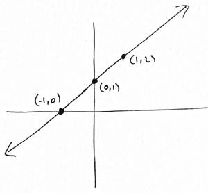
- We can't make a complete list of all solutions, since there are infinitely many solutions in $\mathbb{R}^2$. However, we can draw the set of all solutions as a subset of $\mathbb{R}^2$. This turns out to be a straight line

- $2x+5y=7$ is a linear equation in two variables.
Definition
If $a,b,c$ are any fixed numbers, then equation \[ ax+by=c\] is a linear equation in two variables.
When you draw the set of all solutions of a linear equation in two variables, you always get a straight line in the $x$-$y$ plane.
More examples of linear equations in two variables
- $y-x=1$
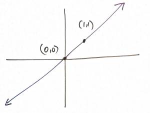
- $x-y=0$
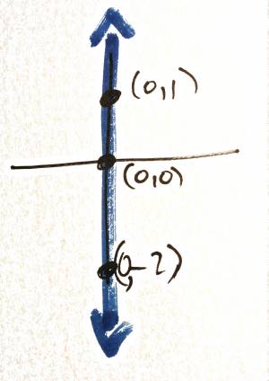
- $x=0\iff 1x+0y=0$
Linear equations in 3 variables
Definition
If $a,b,c,d$ are any fixed numbers, then equation \[ ax+by+cz=d\] is a linear equation in 3 variables.
When you draw the set of all solutions of a linear equation in 3 variables, you always get a plane in 3-dimensional space, $\mathbb{R}^3$.
Examples
- $x+y+z=1$ <html><iframe scrolling=“no” src=“https://tube.geogebra.org/material/iframe/id/528999/width/800/height/503/border/888888/rc/true/ai/false/sdz/true/smb/false/stb/true/stbh/true/ld/false/sri/true/at/auto” width=“800px” height=“503px” style=“border:0px;”> </iframe></html>
- $x+y=1$ This may be viewed as a linear equation in 3 variables, since it is equivalent to $x+y+0z=1$. <html><iframe scrolling=“no” src=“https://tube.geogebra.org/material/iframe/id/529043/width/800/height/503/border/888888/rc/true/ai/false/sdz/true/smb/false/stb/true/stbh/true/ld/false/sri/true/at/auto” width=“800px” height=“503px” style=“border:0px;”> </iframe></html>
- $z=1$, viewed as the equation $0x+0y+z=1$ <html><iframe scrolling=“no” src=“https://tube.geogebra.org/material/iframe/id/529069/width/800/height/503/border/888888/rc/true/ai/false/sdz/true/smb/false/stb/true/stbh/true/ld/false/sri/true/at/auto” width=“800px” height=“503px” style=“border:0px;”> </iframe><br /></html>This plane is horizontal (parallel to the $x$-$y$ plane).
Linear equations (in general)
A linear equation in $m$ variables (where $m$ is some natural number) is an equation of the form \[ a_1x_1+a_2x_2+\dots+a_mx_m=b\] where $a_1,a_2,\dots,a_m$ and $b$ are fixed numbers (called coefficients) and $x_1,x_2,\dots,x_m$ are variables.
Example
\[ 3x_1+5x_2-7x_3+11x_4=12\] is a linear equation in 4 variables.
- A typical solution will be a point $(x_1,x_2,x_3,x_4)\in \mathbb{R}^4$ so that $3x_1+5x_2-7x_3+11x_4$ really does equal $12$.
- For example, $(-2,0,-1,1)$ is a solution.
- The set of all solutions is a 3-dimensional object in $\mathbb{R}^4$, called a hyperplane.
- Since we can't draw pictures in 4-dimensional space $\mathbb{R^4}$ we can't draw this set of solutions!
Systems of linear equations
A system of linear equations is just a list of several linear equations. By a solution of the system, we mean a common solution of each equation in the system.
Example
Find the line of intersection of the two planes $ x+3y+z=5$ and $ 2x+7y+4z=17$.
- <html><iframe scrolling=“no” src=“https://tube.geogebra.org/material/iframe/id/529147/width/800/height/503/border/888888/rc/true/ai/false/sdz/true/smb/false/stb/true/stbh/true/ld/false/sri/true/at/auto” width=“800px” height=“503px” style=“border:0px;”> </iframe></html>
Intersection of $ x+3y+z=5$ and $ 2x+7y+4z=17$
- To find the equation of the line of intersection, we must find the points which are solutions of both equations at the same time.
- Eliminating variables, we get $x=-16+5z$, $y=7-2z$
- The line of intersection consists of the points $(-16+5z,7-2z,z)$, where $z\in\mathbb{R}$
A detailed look at the last example
- $\begin{array}{ccccccrrr} x&+&3y&+&z&=&5&\quad&(1)\\ 2x&+&7y&+&4z&=&17&&(2)\end{array}$
- Find solutions of this system by applying operations
- Aim to end up with a very simple sort of system where we can see the solutions easily.
- $\begin{array}{ccccccrrr} x&+&3y&+&z&=&5&\quad&(1)\\ 2x&+&7y&+&4z&=&17&&(2)\end{array}$
- Replace equation (2) with $(2)-2\times (1)$:
- $\begin{array}{ccccccrrr} x&+&3y&+&z&=&5&\quad&(1)\\ &&y&+&2z&=&7&&(2)\end{array}$
- Now replace equation (1) with $(1)-3\times (2)$
- $\begin{array}{ccccccrrr} x&&&-&5z&=&-16&\quad&(1)\\ &&y&+&2z&=&7&&(2)\end{array}$
- $\begin{array}{ccccccrrr} x&&&-&5z&=&-16&\quad&(1)\\ &&y&+&2z&=&7&&(2)\end{array}$
- can easily rearrange (1) to find $x$ in terms of $z$
- can easily rearrange (2) to find $y$ in terms of $z$
- Since $z$ can take any value, write $z=t$ where $t$ is a “free parameter”
- (which means $t$ can be any real number, or $t\in \mathbb{R}$).
- Solution: \begin{align*} x&=-16+5t\\ y&=7-2t\\ z&=t,\qquad t\in \mathbb{R}\end{align*}
- Solution: \begin{align*} x&=-16+5t\\ y&=7-2t\\ z&=t,\qquad t\in \mathbb{R}\end{align*}
- Can also write this in “vector form”:
- $\begin{bmatrix} x\\y\\z\end{bmatrix}=\begin{bmatrix} -16\\7\\0\end{bmatrix}+t\begin{bmatrix} 5\\-2\\1\end{bmatrix},\qquad t\in \mathbb{R}.$
- This is the equation of the line where the two planes described by the original equations intersect.
- $\begin{bmatrix} x\\y\\z\end{bmatrix}=\begin{bmatrix} -16\\7\\0\end{bmatrix}+t\begin{bmatrix} 5\\-2\\1\end{bmatrix},\qquad t\in \mathbb{R}$
- For each value of $t$, we get a different solution (a different point on the line of intersection).
- e.g. take $t=0$ to see that $(-16,7,0)$ is a solution
- take $t=1.5$ to see that $(-16+1.5\times 5,7+1.5\times (-2),1.5) = (-8.5,4,1.5)$ is another solution
- etc.
- This works for any value $t\in\mathbb{R}$, and every solution may be written in this way.
Another look at the last example
- $\begin{array}{ccccccrrr} x&+&3y&+&z&=&5&\quad&(1)\\ 2x&+&7y&+&4z&=&17&&(2)\end{array}$
- Find solutions of this system by applying operations
- Aim to end up with a very simple sort of system where we can see the solutions easily.
- $\begin{array}{ccccccrrr} x&+&3y&+&z&=&5&\quad&(1)\\ 2x&+&7y&+&4z&=&17&&(2)\end{array}$
- Replace equation (2) with $(2)-2\times (1)$:
- $\begin{array}{ccccccrrr} x&+&3y&+&z&=&5&\quad&(1)\\ &&y&+&2z&=&7&&(2)\end{array}$
- Now replace equation (1) with $(1)-3\times (2)$
- $\begin{array}{ccccccrrr} x&&&-&5z&=&-16&\quad&(1)\\ &&y&+&2z&=&7&&(2)\end{array}$
- $\begin{array}{ccccccrrr} x&&&-&5z&=&-16&\quad&(1)\\ &&y&+&2z&=&7&&(2)\end{array}$
- can easily rearrange (1) to find $x$ in terms of $z$
- can easily rearrange (2) to find $y$ in terms of $z$
- Since $z$ can take any value, write $z=t$ where $t$ is a “free parameter”
- (which means $t$ can be any real number, or $t\in \mathbb{R}$).
- Solution: \begin{align*} x&=-16+5t\\ y&=7-2t\\ z&=t,\qquad t\in \mathbb{R}\end{align*}
- Solution: \begin{align*} x&=-16+5t\\ y&=7-2t\\ z&=t,\qquad t\in \mathbb{R}\end{align*}
- Can also write this in “vector form”:
- $\begin{bmatrix} x\\y\\z\end{bmatrix}=\begin{bmatrix} -16\\7\\0\end{bmatrix}+t\begin{bmatrix} 5\\-2\\1\end{bmatrix},\qquad t\in \mathbb{R}.$
- This is the equation of the line where the two planes described by the original equations intersect.
- $\begin{bmatrix} x\\y\\z\end{bmatrix}=\begin{bmatrix} -16\\7\\0\end{bmatrix}+t\begin{bmatrix} 5\\-2\\1\end{bmatrix},\qquad t\in \mathbb{R}$
- For each value of $t$, we get a different solution (a different point on the line of intersection).
- e.g. take $t=0$ to see that $(-16,7,0)$ is a solution
- take $t=1.5$ to see that $(-16+1.5\times 5,7+1.5\times (-2),1.5) = (-8.5,4,1.5)$ is another solution
- etc.
- This works for any value $t\in\mathbb{R}$, and every solution may be written in this way.
Observations
- The operations we applied to the original linear system don't change the set of solutions. This is because each operation is reversible.
- Writing out the variables $x,y,z$ each time is unnecessary:
- erase the variables from the system $$\begin{array}{ccccccrrr} x&+&3y&+&z&=&5&\quad&(1)\\ 2x&+&7y&+&4z&=&17&&(2)\end{array}$$
- write all the numbers in a grid, or a matrix
- we get $\begin{bmatrix} 1&3&1&5\\2&7&4&17\end{bmatrix}$
- System of linear equations: $\begin{array}{ccccccrrr} x&+&3y&+&z&=&5&\quad&(1)\\ 2x&+&7y&+&4z&=&17&&(2)\end{array}$
- $\begin{bmatrix} 1&3&1&5\\2&7&4&17\end{bmatrix}$ is called the augmented matrix of this linear system
- Each row corresponds to one equation.
- Each column corresponds to one variable
- (except the last column, which has the right-hand-sides of the equations)
- Instead of performing operations on equations, we can perform operations on the rows of this matrix.
\begin{align*} \begin{bmatrix} 1&3&1&5\\2&7&4&17\end{bmatrix} &\xrightarrow{R2\to R2-2\times R1} \begin{bmatrix} 1&3&1&5\\0&1&2&7\end{bmatrix} \\[6pt]&\xrightarrow{R1\to R1-3\times R1} \begin{bmatrix} 1&0&-5&-16\\0&1&2&7\end{bmatrix} \end{align*}
- Translate back into equations and solve:
- $\begin{array}{ccccccrrr} x&&&-&5z&=&-16&\quad&(1)\\ &&y&+&2z&=&7&&(2)\end{array}$
- $\begin{bmatrix} x\\y\\z\end{bmatrix}=\begin{bmatrix} -16\\7\\0\end{bmatrix}+t\begin{bmatrix} 5\\-2\\1\end{bmatrix},\qquad t\in \mathbb{R}.$
This method always works:
- take any system of linear equations
- write down a corresponding matrix (the augmented matrix)
- perform reversible operations on the rows of this matrix to get a “nicer” matrix
- write down a new system of linear equations with the same solutions as the original system.
- Hopefully the new system will be easy to solve…
- and the solutions haven't changed, so we'll have solved the original system!
The augmented matrix and elementary operations
Definition
Given a system of linear equations: \begin{align*} a_{11}x_1+a_{12}x_2+\dots+a_{1m}x_m&=b_1\\ a_{21}x_1+a_{22}x_2+\dots+a_{2m}x_m&=b_2\\ \hphantom{a_{11}}\vdots \hphantom{x_1+a_{22}}\vdots\hphantom{x_2+\dots+{}a_{nn}} \vdots\ & \hphantom{{}={}\!} \vdots\\ a_{n1}x_1+a_{n2}x_2+\dots+a_{nm}x_m&=b_n \end{align*} its augmented matrix is \[ \begin{bmatrix} a_{11}&a_{12}&\dots &a_{1m}&b_1\\ a_{21}&a_{22}&\dots &a_{2m}&b_2\\ \vdots&\vdots& &\vdots&\vdots\\ a_{n1}&a_{n2}&\dots &a_{nm}&b_n \end{bmatrix}.\]
The numbers in this matrix are called its entries.
Example
- Find the augmented matrix of the linear system\begin{align*}3x+4y+7z&=2\\x+3z&=0\\y-2z&=5\end{align*}
- We can rewrite it as \begin{align*}3x+4y+7z&=2\\{\color{red}1}x+{\color{red}0y}+3z&=0\\{\color{red}0x}+{\color{red}1}y-2z&=5\end{align*}
- So the augmented matrix is\[ \begin{bmatrix} 3&4&7&2\\1&0&3&0\\0&1&-2&5\end{bmatrix}.\]
Elementary operations on a system of linear equations
Why do elementary operations leave the solutions of systems unchanged?
- We do the same thing to the left hand side and the right hand side of each equation…
- so any solution to the original system will also be a solution to the new system.
- These operations are all reversible (using operations of the same type)…
- so any solution to the new system will also be a solution to the original system.
Elementary row operations on a matrix
Example
Use EROs to find the intersection of the planes \begin{align*} 3x+4y+7z&=2\\x+3z&=0\\y-2z&=5\end{align*}
Solution 1
\begin{align*} \def\go#1#2#3{\left[\begin{smallmatrix}#1\\#2\\#3\end{smallmatrix}\right]} \def\ar#1{\\\xrightarrow{#1}&} &\go{3&4&7&2}{1&0&3&0}{0&1&-2&5} \ar{\text{reorder rows}}\go{1&0&3&0}{0&1&-2&5}{3&4&7&2} \ar{R3\to R3-3R1}\go{1&0&3&0}{0&1&-2&5}{0&4&-2&2} \ar{R3\to R3-4R2}\go{1&0&3&0}{0&1&-2&5}{0&0&6&-18} \ar{R3\to \tfrac16 R3}\go{1&0&3&0}{0&1&-2&5}{0&0&1&-3} \end{align*}
$\go{1&0&3&0}{0&1&-2&5}{0&0&1&-3}$
- from the last row, we get $z=-3$
- from the second row, we get $y-2z=5$
- so $y-2(-3)=5$
- so $y=-1$
- from the first row, we get $x+3z=0$
- so $x+3(-3)=0$
- so $x=9$
- Conclusion: $\begin{bmatrix}x\\y\\z\end{bmatrix}=\begin{bmatrix}9\\-1\\-3\end{bmatrix}$ is the only solution.
Solution 2
We start in the same way, but by performing more EROs we make the algebra at the end simpler.
\begin{align*} \def\go#1#2#3{\left[\begin{smallmatrix}#1\\#2\\#3\end{smallmatrix}\right]} \def\ar#1{\\\xrightarrow{#1}&} &\go{3&4&7&2}{1&0&3&0}{0&1&-2&5} \ar{\ldots \text{same EROs as above}\ldots}\go{1&0&3&0}{0&1&-2&5}{0&0&1&-3} \ar{R2\to R2+2R3}\go{1&0&3&0}{0&1&0&-1}{0&0&1&-3} \ar{R1\to R1-3R3}\go{1&0&0&9}{0&1&0&-1}{0&0&1&-3} \end{align*}
\[ \go{1&0&0&9}{0&1&0&-1}{0&0&1&-3}\]
- from the last row, we get $z=-3$
- from the second row, we get $y=-1$
- from the first row, we get $x=9$
- So $\begin{bmatrix}x\\y\\z\end{bmatrix}=\begin{bmatrix}9\\-1\\-3\end{bmatrix}$ is the only solution.
Discussion
Both solutions use EROs to transform the augmented matrix.
- Solution 1: $\left[\begin{smallmatrix}1&0&3&0\\0&1&-2&5\\0&0&1&-3\end{smallmatrix}\right]$.
- “Staircase pattern”: 1s on “steps”, zeros below steps
- Called row echelon form
- Needed algebra to finish solution.
- Solution 2: $\left[\begin{smallmatrix}1&0&0&9\\0&1&0&-1\\0&0&1&-3\end{smallmatrix}\right]$
- Staircase with zeros above 1s on steps (and below).
- Called reduced row echelon form
- No extra algebra needed to finish solution.