This is an old revision of the document!
Warning: Undefined array key "do" in /home/levene/public_html/w/mst10030/lib/plugins/revealjs/action.php on line 14
Table of Contents
Chapter 1: Systems of linear equations
Linear equations
First example: a linear equation in two variables
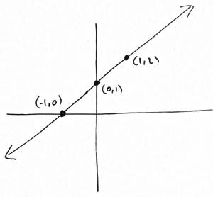
Consider the equation \[ 2x+5y=7.\] This is an equation in two variables, or indeterminates, $x$ and $y$.
A solution of this equation is a pair of numbers $(a,b)\in \mathbb{R}^2$ so that if we replace $x$ with $a$ and replace $y$ with $b$, then the equation becomes true.
In other words, so that $2a+5b$ really is equal to $7$.
- $(3,1)$ is not a solution, because $2\times 3+5\times 1\ne 7$
- $(1,1)$ is a solution, because $2\times 1+5\times 1=7$
- Other solutions include $(0,\tfrac 75)$, $(0.5,1.2)$, $(6,-1)$, $(3.5,0)$, $(-\tfrac32,2)$, …
We can't make a complete list of all solutions, since there are infinitely many solutions in $\mathbb{R}^2$. However, we can draw the set of all solutions as a subset of $\mathbb{R}^2$. This turns out to be a straight line:

We say that the equation $2x+5y=7$ is a linear equation in two variables.
Definition
If $a,b,c$ are any fixed numbers, then equation \[ ax+by=c\] is a linear equation in two variables.
When you draw the set of all solutions of a linear equation in two variables, you always get a straight line in the $x$-$y$ plane.
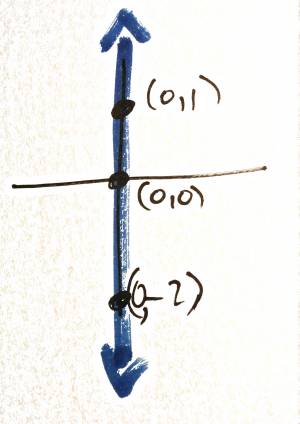
More examples of linear equations in two variables
- $y-x=1$
- $x-y=0$
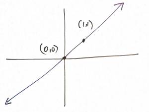
- $x=0\iff 1x+0y=0$
Linear equations in 3 variables
Definition
If $a,b,c,d$ are any fixed numbers, then equation \[ ax+by+cz=d\] is a linear equation in 3 variables.
When you draw the set of all solutions of a linear equation in 3 variables, you always get a plane in 3-dimensional space, $\mathbb{R}^3$.
Examples
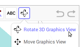
Note: you can view the examples below from different angles, by clicking the “Rotate 3D graphics view” button.
- $x+y+z=1$ <html><iframe scrolling=“no” src=“https://tube.geogebra.org/material/iframe/id/528999/width/800/height/503/border/888888/rc/true/ai/false/sdz/true/smb/false/stb/true/stbh/true/ld/false/sri/true/at/auto” width=“800px” height=“503px” style=“border:0px;”> </iframe></html>
- $x+y=1$ This may be viewed as a linear equation in 3 variables, since it is equivalent to $x+y+0z=1$. <html><iframe scrolling=“no” src=“https://tube.geogebra.org/material/iframe/id/529043/width/800/height/503/border/888888/rc/true/ai/false/sdz/true/smb/false/stb/true/stbh/true/ld/false/sri/true/at/auto” width=“800px” height=“503px” style=“border:0px;”> </iframe></html>
- $z=1$, viewed as the equation $0x+0y+z=1$ <html><iframe scrolling=“no” src=“https://tube.geogebra.org/material/iframe/id/529069/width/800/height/503/border/888888/rc/true/ai/false/sdz/true/smb/false/stb/true/stbh/true/ld/false/sri/true/at/auto” width=“800px” height=“503px” style=“border:0px;”> </iframe><br /></html>This plane is horizontal (parallel to the $x$-$y$ plane).
Linear equations (in general)
A linear equation in $m$ variables (where $m$ is some natural number) is an equation of the form \[ a_1x_1+a_2x_2+\dots+a_mx_m=b\] where $a_1,a_2,\dots,a_m$ and $b$ are fixed numbers (called coefficients) and $x_1,x_2,\dots,x_m$ are variables.
Example
\[ 3x_1+5x_2-7x_3+11x_4=12\] is a linear equation in 4 variables.
- A typical solution will be a point $(x_1,x_2,x_3,x_4)\in \mathbb{R}^4$ so that $3x_1+5x_2-7x_3+11x_4$ really does equal $12$.
- For example, $(-2,0,-1,1)$ is a solution.
- The set of all solutions is a 3-dimensional object in $\mathbb{R}^4$, called a hyperplane.
- Since we can't draw pictures in 4-dimensional space $\mathbb{R^4}$ we can't draw this set of solutions!
Systems of linear equations
A system of linear equations is just a list of several linear equations. By a solution of the system, we mean a common solution of each equation in the system.
Example
Find the line of intersection of the two planes \[ x+3y+z=5\] and \[ 2x+7y+4z=17.\]
Just to get an idea of what's going on, here's a picture of the two planes:
<html><iframe scrolling=“no” src=“https://tube.geogebra.org/material/iframe/id/529147/width/800/height/503/border/888888/rc/true/ai/false/sdz/true/smb/false/stb/true/stbh/true/ld/false/sri/true/at/auto” width=“800px” height=“503px” style=“border:0px;”> </iframe></html>
To find the equation of the line of intersection, we must find the points which are solutions of both equations at the same time. Eliminating variables, we get \[ x=-16+5z,\quad y=7-2z\] which tells us that for any value of $z$, the point \[ (-16+5z,7-2z,z)\] is a typical point in the line of intersection.
Let's look at the example from the end of Lecture 2 more closely: $$\begin{array}{ccccccrrr} x&+&3y&+&z&=&5&\quad&(1)\\ 2x&+&7y&+&4z&=&17&&(2)\end{array}$$ We find the solutions of this system by applying operations to the system to make a new system, aiming to end up with a very simple sort of system where we can see the solutions easily.
First replace equation (2) with $(2)-2\times (1)$. We'll call the resulting equations (1) and (2) again, although of course we end up with a different system of linear equations: $$\begin{array}{ccccccrrr} x&+&3y&+&z&=&5&\quad&(1)\\ &&y&+&2z&=&7&&(2)\end{array}$$ Now replace equation (1) with $(1)-3\times (2)$: $$\begin{array}{ccccccrrr} x&&&-&5z&=&-16&\quad&(1)\\ &&y&+&2z&=&7&&(2)\end{array}$$ Notice that we can now easily rearrange (1) to find $x$ in terms of $z$, and we can rearrange (2) to find $y$ in terms of $z$. Since $z$ can take any value, we write $z=t$ where $t$ is a “free parameter” (which means $t$ can be any real number, or $t\in \mathbb{R}$). \begin{align*} x&=-16+5t\\ y&=7-2t\\ z&=t,\qquad t\in \mathbb{R}\end{align*} We can also write this in so-called “vector form”: \[ \begin{bmatrix} x\\y\\z\end{bmatrix}=\begin{bmatrix} -16\\7\\0\end{bmatrix}+t\begin{bmatrix} 5\\-2\\1\end{bmatrix},\qquad t\in \mathbb{R}.\] This is the equation of the line where the two planes described by the original equations (1) and (2) intersect.
Note for each different value of $t$, we get a different solutions (that is, a different point on the line of intersection). For example, setting $t=0$ we see that $(-16,7,0)$ is a solution; setting $t=1.5$, we see that $(-16+1.5\times 5,7+1.5\times (-2),1.5) = (-8.5,4,1.5)$ is another solution, and so on. This works for any value $t\in\mathbb{R}$, and every solution may be written in this way.
Observations
- The operations we applied to the original linear system don't change the set of solutions. This is because each operation is reversible.
- Writing out the variables $x,y,z$ each time is unnecessary. If we erase the variables from the system $$\begin{array}{ccccccrrr} x&+&3y&+&z&=&5&\quad&(1)\\ 2x&+&7y&+&4z&=&17&&(2)\end{array}$$ and write all the numbers in a grid, or a matrix, we get:
\[ \begin{bmatrix} 1&3&1&5\\2&7&4&17\end{bmatrix}\] Notice that the first column corresponds to the $x$ variable, the second to $y$, the third to $z$ and the numbers in the final column are the right hand sides of the equations. Each row corresponds to one equation. So instead of performing operations on equations, we can perform operations on the rows of this matrix: \begin{align*} &\begin{bmatrix} 1&3&1&5\\2&7&4&17\end{bmatrix} \\[6pt]\xrightarrow{R2\to R2-2\times R1}& \begin{bmatrix} 1&3&1&5\\0&1&2&7\end{bmatrix} \\[6pt]\xrightarrow{R1\to R1-3\times R1}& \begin{bmatrix} 1&0&-5&-16\\0&1&2&7\end{bmatrix} \end{align*} Now we translate this back into equations to solve: $$\begin{array}{ccccccrrr} x&&&-&5z&=&-16&\quad&(1)\\ &&y&+&2z&=&7&&(2)\end{array}$$ so \[ \begin{bmatrix} x\\y\\z\end{bmatrix}=\begin{bmatrix} -16\\7\\0\end{bmatrix}+t\begin{bmatrix} 5\\-2\\1\end{bmatrix},\qquad t\in \mathbb{R}.\]
This sort of thing works in general: we can take any system of linear equations, write down a corresponding matrix, perform certain reversible operations on the rows of this matrix to get a new matrix, and then write down a new system of linear equations with the same solutions as the original system. If we do things in a sensible way then the new system will be easy to solve, so we'll be able to solve the original system (since the solution set is the same).
Let's give some terminology which will allow us to make this process clear.
The augmented matrix of a system of linear equations
Definition
Given a system of linear equations: \begin{align*} a_{11}x_1+a_{12}x_2+\dots+a_{1m}x_m&=b_1\\ a_{21}x_1+a_{22}x_2+\dots+a_{2m}x_m&=b_2\\ \hphantom{a_{11}}\vdots \hphantom{x_1+a_{22}}\vdots\hphantom{x_2+\dots+{}a_{nn}} \vdots\ & \hphantom{{}={}\!} \vdots\\ a_{n1}x_1+a_{n2}x_2+\dots+a_{nm}x_m&=b_n \end{align*} its augmented matrix is \[ \begin{bmatrix} a_{11}&a_{12}&\dots &a_{1m}&b_1\\ a_{21}&a_{22}&\dots &a_{2m}&b_2\\ \vdots&\vdots& &\vdots&\vdots\\ a_{n1}&a_{n2}&\dots &a_{nm}&b_n \end{bmatrix}.\]
The numbers in this matrix are called the entries of the matrix. We can be a bit more precise: the number in row $i$ and column $j$ is called the $(i,j)$ entry of the matrix.
Example
To find the augmented matrix of the linear system \begin{align*} 3x+4y+7z&=2\\x+3z&=0\\y-2z&=5 \end{align*} notice that we can rewrite it as \begin{align*} 3x+4y+7z&=2\\{\color{red}1}x+{\color{red}0y}+3z&=0\\{\color{red}0x}+{\color{red}1}y-2z&=5 \end{align*} so the augmented matrix is \[ \begin{bmatrix} 3&4&7&2\\1&0&3&0\\0&1&-2&5\end{bmatrix}.\]
- the $(2,3)$ entry of this matrix is $3$;
- the $(3,2)$ entry is $1$;
- the $(1,4)$ entry is $2$;
- the $(4,1)$ entry is undefined (since this matrix does not have a $4$th row).
Elementary operations on a system of linear equations
If we perform one of the following operations on a system of linear equations:
- list the equations in a different order; or
- multiply one of the equations by a non-zero real number; or
- replace equation $j$ by “equation $j$ ${}+{}$ $c\times {}$ (equation $i$)”, where $c$ is a non-zero real number,
then the new system will have exactly the same solutions as the original system. These are called elementary operations on the linear system.
Why do elementary operations leave the solutions of systems unchanged?
- we are doing the same thing to the left hand side and the right hand side of each equation, so any solution to the original system will also be a solution to the new system; and
- these operations are reversible, using operations of the same type, so any solution to the new system will also be a solution to the original system.
Elementary row operations on a matrix
Recall that when we form the augmented matrix of a linear system, each equation in the system becomes a row of the matrix. So we can translate the elementary operations on the linear system into corresponding operations on the rows of the matrix. We get three different types:
- change the order of the rows of the matrix;
- multiply one of the rows of the matrix by a non-zero real number;
- replace row $j$ by “row $j$ ${}+{}$ $c\times {}$ (row $i$)”, where $c$ is a non-zero real number and $i\ne j$.
The system of linear equations corresponding to these matrices will then have exactly the same solutions.
We call these operations elementary row operations or EROs on the matrix.
Example
Use EROs to find the intersection of the planes \begin{align*} 3x+4y+7z&=2\\x+3z&=0\\y-2z&=5\end{align*}
Solution 1
\begin{align*} \def\go#1#2#3{\begin{bmatrix}#1\\#2\\#3\end{bmatrix}} \def\ar#1{\\[6pt]\xrightarrow{#1}&} &\go{3&4&7&2}{1&0&3&0}{0&1&-2&5} \ar{\text{reorder rows}}\go{1&0&3&0}{0&1&-2&5}{3&4&7&2} \ar{R3\to R3-3R1}\go{1&0&3&0}{0&1&-2&5}{0&4&-2&2} \ar{R3\to R3-4R2}\go{1&0&3&0}{0&1&-2&5}{0&0&6&-18} \ar{R3\to \tfrac16 R3}\go{1&0&3&0}{0&1&-2&5}{0&0&1&-3} \end{align*}
So
- from the last row, we get $z=-3$
- from the second row, we get $y-2z=5$, so $y-2(-3)=5$, so $y=-1$
- from the first row, we get $x+3z=0$, so $x+3(-3)=0$, so $x=9$
The conclusion is that \[ \begin{bmatrix}x\\y\\z\end{bmatrix}=\begin{bmatrix}9\\-1\\-3\end{bmatrix}\] is the only solution.
Solution 2
We start in the same way, but by performing more EROs we make the algebra at the end simpler.
\begin{align*} \def\go#1#2#3{\begin{bmatrix}#1\\#2\\#3\end{bmatrix}} \def\ar#1{\\[6pt]\xrightarrow{#1}&} &\go{3&4&7&2}{1&0&3&0}{0&1&-2&5} \ar{\text{reorder rows}}\go{1&0&3&0}{0&1&-2&5}{3&4&7&2} \ar{R3\to R3-3R1}\go{1&0&3&0}{0&1&-2&5}{0&4&-2&2} \ar{R3\to R3-4R2}\go{1&0&3&0}{0&1&-2&5}{0&0&6&-18} \ar{R3\to \tfrac16 R3}\go{1&0&3&0}{0&1&-2&5}{0&0&1&-3} \ar{R2\to R2+2R3}\go{1&0&3&0}{0&1&0&-1}{0&0&1&-3} \ar{R1\to R1-3R3}\go{1&0&0&9}{0&1&0&-1}{0&0&1&-3} \end{align*}
So
- from the last row, we get $z=-3$
- from the second row, we get $y=-1$
- from the first row, we get $x=9$
The conclusion is again that \[ \begin{bmatrix}x\\y\\z\end{bmatrix}=\begin{bmatrix}9\\-1\\-3\end{bmatrix}\] is the only solution.
Discussion
In both of these solutions we used EROs to transform the augmented matrix into a nice form.
- In solution 1, we ended up with the matrix $\left[\begin{smallmatrix}1&0&3&0\\0&1&-2&5\\0&0&1&-3\end{smallmatrix}\right]$ which has a staircase pattern, with zeros below the staircase, and 1s just above the “steps” of the staircase. This is an example of a matrix in row echelon form (see below). We needed a bit of easy algebra, called back substitution, to finish off the solution. (Why is it called echelon form? It seems that this word has an archaic meaning which is relevant to the staircase-like pattern: “any structure or group of structures arranged in a steplike form.”)
- In solution 2, we ended up with the matrix $\left[\begin{smallmatrix}1&0&0&9\\0&1&0&-1\\0&0&1&-3\end{smallmatrix}\right]$ which has a staircase pattern with zeros below the staircase and 1s just above the “steps” of the staircase, and the additional property that we only have zeros above the 1s on the steps. This is an example of a matrix in reduced row echelon form (see below). Finding the solution from this matrix needed no extra algebra.
Row echelon form and reduced row echelon form
Row echelon form (REF)
Definition
A row of a matrix is a zero row if it contains only zeros. For example, $[0\ 0\ 0\ 0\ 0]$ is a zero row.
A row of a matrix is non-zero, or a non-zero row if contains at least one entry that is not $0$. For example $[0\ 0\ 3\ 0\ 0]$ is non-zero, and so is $[1\ 2\ 3\ 4\ -5]$.
Definition
The leading entry of a non-zero row of a matrix is the leftmost entry which is not $0$.
For example, the leading entry of the row $[0~0~0~6~2~0~3~1~0]$ is $6$.
Definition
A matrix is in row echelon form, or REF, if it has all of the following three properties:
- The zero rows of the matrix (if any) are all at the bottom of the matrix.
- In every non-zero row of the matrix, the leading entry is $1$.
- If row $i$ and row $(i+1)$ are both non-zero, then the leading entry in row $(i+1)$ is to the right of the leading entry in row $i$. <html><br /></html>In other words, as you go down the rows, the leading entries must go to the right.
For example, $\left[\begin{smallmatrix} 1&2&3&4&5\\0&1&2&3&4\\0&0&1&2&3\end{smallmatrix}\right]$ and $\left[\begin{smallmatrix} 1&2&3&4&5\\0&1&2&3&4\\0&0&1&2&3\\0&0&0&0&0\end{smallmatrix}\right]$ are both in REF, but
- $\left[\begin{smallmatrix} 1&2&3&4&5\\0&0&0&0&0\\0&0&1&2&3\end{smallmatrix}\right]$ and $\left[\begin{smallmatrix} 1&2&3&4&5\\0&0&0&0&0\\0&0&1&2&3\\0&0&0&0&0\end{smallmatrix}\right]$ are not in REF, since they each have a zero row which isn't at the bottom;
- $\left[\begin{smallmatrix} 1&2&3&4&5\\0&2&3&4&1\\0&0&1&2&3\end{smallmatrix}\right]$ is not in REF, since the leading entry on the second row isn't $1$;
- $\left[\begin{smallmatrix} 0&1&2&3&4\\1&2&3&4&5\\0&0&1&2&3\end{smallmatrix}\right]$ is not in REF, since the leading entry in row $2$ is not to the right of the leading entry in row $1$.
Reduced row echelon form (RREF)
Definition
A matrix is in reduced row echelon form or RREF if it is in row echelon form (REF), so that
- The zero rows of the matrix (if any) are all at the bottom of the matrix.
- In every non-zero row of the matrix, the leading entry is $1$.
- If row $i$ and row $(i+1)$ are both non-zero, then the leading entry in row $(i+1)$ is to the right of the leading entry in row $i$. <html><br /></html>In other words, as you go down the rows, the leading entries must go to the right.
and the matrix also has the property:
<html><ol start=“4”><li class=“level1”><div class=“li”></html> If a column contains the leading entry of a row, then every other entry in that column is $0$. <html></div></li></ol></html>
For example, \[\begin{bmatrix} {\color{blue}1}&{\color{red}2}&{\color{red}3}&4&5\\0&{\color{blue}1}&{\color{red}2}&3&4\\0&0&{\color{blue}1}&2&3\end{bmatrix}\quad\text{and}\quad \begin{bmatrix} {\color{blue}1}&0&{\color{red}3}&4&5\\0&{\color{blue}1}&0&3&4\\0&0&{\color{blue}1}&2&3\end{bmatrix}\] are both in REF, but they are not in RREF because the red entries are non-zero and are in the same column as a leading entry (in blue).
On the other hand, \[\begin{bmatrix} {\color{blue}1}&0&0&4&5\\0&{\color{blue}1}&0&3&4\\0&0&{\color{blue}1}&2&3\end{bmatrix}\] is in RREF.
Example
Use EROs to put the following matrix into RREF: \[\begin{bmatrix} 1&2&3&4&5\\0&1&2&3&4\\0&0&1&2&3\end{bmatrix}\] and solve the corresponding linear system.
Solution
\begin{align*} \def\go#1#2#3{\begin{bmatrix}#1\\#2\\#3\end{bmatrix}} \def\ar#1{\\[6pt]\xrightarrow{#1}&} &\go{1&2&3&4&5}{0&1&2&3&4}{0&0&1&2&3} \ar{R2\to R2-2R3}\go{1&2&3&4&5}{0&1&0&-1&-2}{0&0&1&2&3} \ar{R1\to R1-3R3}\go{1&2&0&-2&-4}{0&1&0&-1&-2}{0&0&1&2&3} \ar{R1\to R1-2R2}\go{1&0&0&0&0}{0&1&0&-1&-2}{0&0&1&2&3} \end{align*} This matrix is in RREF. Write $x_i$ for the variable corresponding to the $i$th column. The solution is
- $x_4=t$, a free parameter, i.e. $t\in\mathbb{R}$. This is because the $4$th column does not contain a leading entry.
- From row 3: $x_3+2t=3$, so $x_3=3-2t$
- From row 2: $x_2-t=-2$, so $x_2=-2+t$
- From row 1: $x_1=0$
So the solution is \[ \begin{bmatrix}x_1\\x_2\\x_3\\x_4\end{bmatrix}=\begin{bmatrix}0\\-2\\3\\0\end{bmatrix}+ t\begin{bmatrix}0\\1\\-2\\1\end{bmatrix},\quad t\in\mathbb{R}.\]
(Geometrically, this is a line in 4-dimensional space $\mathbb{R}^4$).